2 Single Degree of Freedom Systems
Learning Outcomes
By the end of this chapter, students will be able to:
- Describe the free vibration motion of an undamped spring-mass system and define its natural frequency
- Represent oscillatory motion using a complex exponential and relate the complex amplitude to the phase angle
- Describe the natural frequency and damping ratio of a spring-mass-damper system and classify its free vibration response as overdamped, critically damped or underdamped
- Describe the harmonically forced vibration motion of a single degree of freedom system, including its homogeneous and particular solutions
- Derive and interpret the response amplitude operator (RAO) of a single degree of freedom system, including the phenomena of resonance and phase lag
- Explain the principle of superposition for linear systems and apply it to compute the response to a multi-frequency excitation
- Derive the hydrostatic restoring stiffness and heave natural frequency of a freely floating body
2.1 Motivation
A ship or an offshore platform operating in the open ocean is free to more in all six degrees of freedom and experiences forces due to the random waves, wind and currents in the ocean. While we embark on this journey to be able to analyze this problem by the end of the course, let’s start small by understanding the dynamics of a simple spring-mass-damper system. We will later see that some of the concepts we learn with respect to this simplified system transfer over to our ship or floating platform dyanmics too.
2.2 Spring mass system - Free vibration
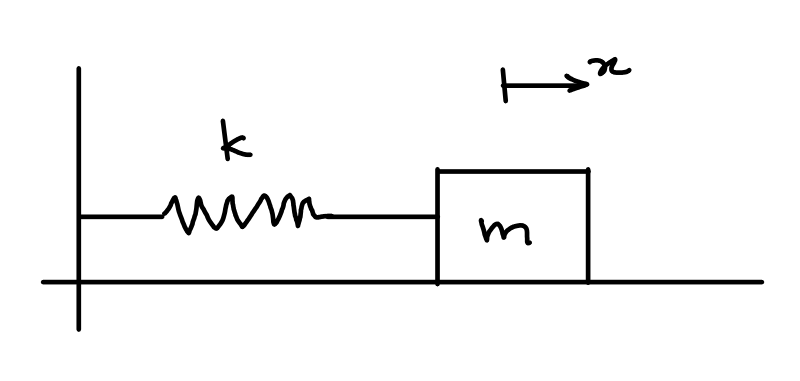
Consider a mass on a flat surface connected to a massless spring as shown in Figure 2.1. The mass is free to move in the horizontal direction. One end of the spring is attached to the mass and the other end of the spring is attached to a fixed point. We will assume that the surface is frictionless. We denote the displacement of the mass from its equilibrium position as \(x(t)\).
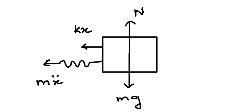
The free body diagram of the spring mass system is shown in Figure 2.2. The equilibrium of forces along horizontal and vertical axes yields:
\[\begin{align} m \frac{d^2x}{dt^2} + kx = 0 \\ mg = N \end{align}\]
The first equation can be recast as:
\[\begin{align} \frac{d^2x}{dt^2} + \omega_n^2 x = 0 \label{eq-sdof-spring-mass-eom} \end{align}\]
where \(\omega_n\) is the natural frequency of the system and is denoted by:
\[\begin{align} \omega_n = \sqrt{\frac{k}{m}} \end{align}\]
It is easy to see that the solution to \(\eqref{eq-sdof-spring-mass-eom}\) is:
\[\begin{align} x(t) = A \cos(\omega_n t) + B \sin(\omega_n t) \label{eq-sdof-undamped-gen-sol} \end{align}\]
The constants \(A\) and \(B\) can be determined from the specified initial conditions. If the initial displacement is \(x(0) = x_0\) and initial velocity is \(\dot{x}(0) = v_0\), then the solution in terms of the initial conditions is given by:
\[\begin{align} x(t) = x_0 \cos(\omega_n t) + \frac{v_0}{\omega_n} \sin(\omega_n t) \end{align}\]
We can see that the solution persists indefinitely for a non-zero initial condition.
Common Pitfall
Note that the initial condition has no influence on the natural frequency of the system. The natural frequency is only dependent on the mass \(m\) and stiffness \(k\).
Interactive Simulation
Use the tool below to explore how the mass \(m\), stiffness \(k\), initial displacement \(x_0\) and initial velocity \(v_0\) affect the free vibration response of the spring mass system. The 3D animation shows the physical motion of the mass, while the plots track the displacement time history, velocity time history, and the phase space trajectory (\(x\) vs. \(\dot{x}\)).
Displacement vs Time
Velocity vs Time
Phase Space
2.3 Complex response
We saw that in the previous section, both \(x_1(t) = \cos(\omega_n t)\) and \(x_2(t) = \sin(\omega_n t)\) satisfy the differential equation \(\eqref{eq-sdof-spring-mass-eom}\). Both these solutions can be combined together using the Euler’s identity as:
\[\begin{align} x_c(t) = x_1(t) + i x_2(t) = \cos(\omega_n t) + i \sin(\omega_n t) = e^{i \omega_n t} \end{align}\]
We can see that the complex response \(x_c(t)\) also satisfies the differential equation \(\eqref{eq-sdof-spring-mass-eom}\). The notion of a complex response for a spring-mass system may seem odd at first. However, we will see its usefulness in a bit. Let’s assume a general solution of the form:
\[\begin{align} x_c(t) = A_c e^{i \omega_n t} \end{align}\]
where \(A_c\) is complex valued amplitude. The complex amplitude \(A_c\) can be related back to the real coefficients \(A\) and \(B\) as:
\[\begin{align} A_c &= \sqrt{A^2 + B^2} e^{i\phi} \quad \text{where} \quad \phi = \tan^{-1}{\left(\frac{-B}{A}\right)} \\ &= A - iB \end{align}\]
\(\phi\) is called the phase angle and its importance will be evident when we discuss the forced vibration of a spring mass system. It can be seen that the real part of this complex response is:
\[\begin{align} x_r(t) &= \operatorname{Re}(x_c(t)) = \operatorname{Re}\left(\sqrt{A^2 + B^2} e^{i(\omega_n t + \phi)}\right) = \sqrt{A^2 + B^2} \cos{(\omega_n t + \phi)} \nonumber \\ &= \sqrt{A^2 + B^2} \left(\cos(\omega_n t) \cos(\phi) - \sin(\omega_n t) \sin(\phi) \right) \nonumber \\ &= A \cos(\omega_n t) + B \sin(\omega_n t) \end{align}\]
the same as we saw in \(\eqref{eq-sdof-undamped-gen-sol}\). The complex response in terms of the initial conditions can be expressed as:
\[\begin{align} x_c(t) = \left(x_0 - \frac{iv_0}{\omega_n} \right) e^{i \omega_n t} \end{align}\]
2.4 Spring mass damper system - Free vibration
Now let’s add a dashpot to our system that provides damping to the system as seen in Figure 2.3. The corresponding free body diagram is now shown in Figure 2.4.
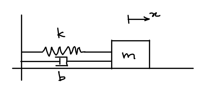
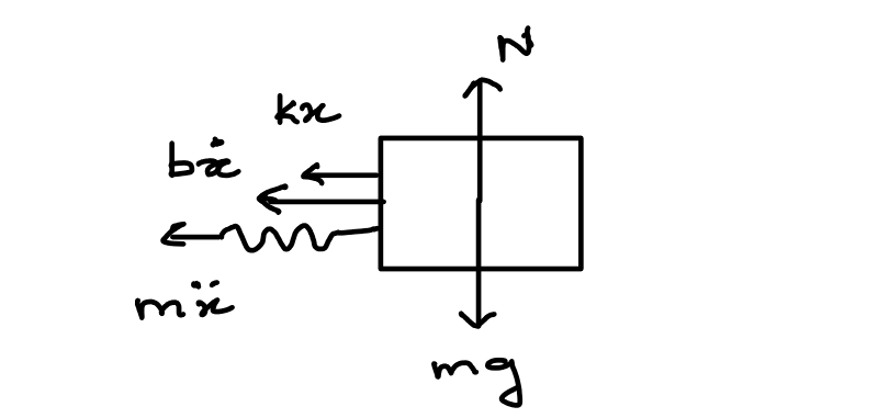
The equilibrium of forces along the horizontal direction gives us the equation of motion as:
\[\begin{align} m \frac{d^2x}{dt^2} + b \frac{dx}{dt} + kx = 0 \\ \end{align}\]
This equation can be recast as:
\[\begin{align} \frac{d^2x}{dt^2} + 2\zeta\omega_n\frac{dx}{dt} + \omega_n^2 x = 0 \label{eq-sdof-smd-eom} \end{align}\]
where \(\omega_n\) is the natural frequency of the system and \(\zeta\) is the damping ratio denoted by:
\[\begin{align} \zeta = \frac{b}{2\sqrt{mk}} \end{align}\]
It is easy to see now that \(e^{i\omega_n t}\) no longer satisfies the differential equation \(\eqref{eq-sdof-smd-eom}\). Thus, we assume a general solution of the form:
\[\begin{align} x_c(t) = A_c e^{i \omega t} \end{align}\]
where we do not yet know the \(\omega\). Note that we choose the exponential function as the differential equation \(\eqref{eq-sdof-smd-eom}\) is still linear. Substituting into the differential equation yields:
\[\begin{align} \left(-\omega^2 + i2\zeta\omega_n\omega + \omega_n^2\right) A_c e^{i \omega t} = 0 \end{align}\]
We are interested in the non-trivial solution (\(A_c \neq 0\)) and that leads to the quadratic equation:
\[\begin{align} -\omega^2 + i2\zeta\omega_n\omega + \omega_n^2 = 0 \end{align}\]
with the roots:
\[\begin{align} \omega_{1,2} = i\zeta \omega_n \pm \omega_n \sqrt{1 - \zeta^2} \end{align}\]
Thus the general solution for the spring mass damper system is given by:
\[\begin{align} x_c(t) &= A_c e^{i\omega_1 t} + B_c e^{i\omega_2 t} \\ &= e^{-\zeta \omega_n t} \left(A_c e^{i\omega_nt\sqrt{1 - \zeta^2}} + B_c e^{-i\omega_nt\sqrt{1 - \zeta^2}} \right) \end{align}\]
Now there are three possible scenarios:
- Overdamped scenario \(\zeta > 1\)
- Critically damped scenario \(\zeta = 1\)
- Underdamped scenario \(\zeta < 1\)
Overdamped case
In this case, we see that the \(\sqrt{1 - \zeta^2} = i\sqrt{\zeta^2 - 1}\) and the general solution takes the form:
\[\begin{align} x_c(t) &= A_c e^{\omega_nt(-\zeta - \sqrt{\zeta^2 - 1})} + B_c e^{\omega_nt(-\zeta + \sqrt{\zeta^2 -1})} \end{align}\]
The coefficients of time for both exponents are negative and real. This leads to the solution \(x_c(t) \rightarrow 0\) as \(t \rightarrow 0\). Note that for the overdamped case \(A_c\) and \(B_c\) are real valued.
Critically damped case
In this case we have repeated roots \(\omega_1 = \omega_2 = i \omega_n\). The solution \(x_c(t)\) in this case takes the form:
\[\begin{align} x_c(t) = A_c e^{-\omega_nt} + B_c te^{-\omega_nt} \end{align}\]
Note that in the case of critically damped case, both homogeneous solutions become the same upon substituting \(\zeta = 1\). However, since the system is described a second order differential equation, two homogeneous solutions will exist. A second homogeneous solution exists of the form \(te^{-\omega_n t}\) and it can be seen that it satisfies the differential equation.
As before in the overdamped case, here too both terms have negative time coefficients in the exponential terms and the solution \(x_c(t) \rightarrow 0\) as \(t \rightarrow 0\). Note that for the critically damped case \(A_c\) and \(B_c\) are real valued.
Underdamped case
In this case the system exhibits an oscillatory response. The response reduces to the form:
\[\begin{align} x_c(t) &= e^{-\zeta \omega_n t} \left(A_c e^{i\omega_dt} + B_c e^{-i\omega_dt}\right) \end{align}\]
where \(\omega_d = \omega_n \sqrt{1-\zeta^2}\) is the damped natural frequency. The real part of the solution can be expressed as:
\[\begin{align} x_r(t) &= e^{-\zeta \omega_n t} \left(A \cos(\omega_dt) + B \sin(\omega_dt) \right) \end{align}\]
The coefficients \(A\) and \(B\) are determined as before from the initial conditions. If the initial conditions are \(x_r(0) = x_0\) and \(\dot{x}_r = v_0\), then the solution in terms of the initial conditions can be expressed as:
\[\begin{align} x_r(t) = e^{-\zeta \omega_n t} \left(x_0 \cos(\omega_dt) + \frac{v_0 + \zeta\omega_nx_0}{\omega_d} \sin(\omega_dt) \right) \end{align}\]
Interactive Simulation
Use the tool below to explore how the natural frequency \(\omega_n\) and damping ratio \(\zeta\) affect the free vibration response of the spring mass damper system. Drag the damping ratio slider across \(\zeta = 1\) to move between the underdamped, critically damped and overdamped regimes. The 3D animation shows the physical motion of the mass, while the plots track the displacement time history (with its decay envelope shown as a dashed line when underdamped), velocity time history, and the phase space trajectory (\(x\) vs. \(\dot{x}\)).
Displacement vs Time
Velocity vs Time
Phase Space
2.5 Spring mass damper system - Forced vibration
Now let’s consider that an external force \(F(t) = F_0 \cos(\omega t) = \operatorname{Re}(F_0 e^{i\omega t})\) acting on the mass as seen in Figure 2.5. The corresponding free body diagram is now shown in Figure 2.6.
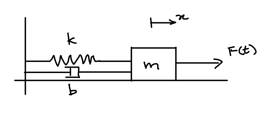
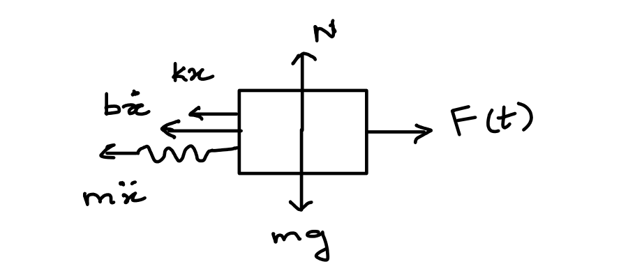
The equilibrium of forces along the horizontal direction gives us the equation of motion as:
\[\begin{align} m \frac{d^2x}{dt^2} + b \frac{dx}{dt} + kx = F_0 \cos(\omega t) \\ \end{align}\]
This equation can be recast as:
\[\begin{align} \frac{d^2x}{dt^2} + 2\zeta\omega_n\frac{dx}{dt} + \omega_n^2 x = f_0 \cos(\omega t) \label{eq-sdof-smd-forced-eom} \end{align}\]
where \(f_0 = F_0/m\). Assuming a particular solution of the form \(x_c(t) = A_c e^{i\omega t}\) and substituting it into \(\eqref{eq-sdof-smd-forced-eom}\) yields:
\[\begin{align} \left(-\omega^2 + i2\zeta\omega_n\omega + \omega_n^2\right)A_c e^{i\omega t} = f_0 e^{i\omega t} \end{align}\]
For a non-trivial solution (\(A_c \neq 0\)):
\[\begin{align} A_c = \frac{F_0/k}{\left(1 - \frac{\omega^2}{\omega_n^2}\right) + i 2 \zeta \frac{\omega}{\omega_n}} \end{align}\]
The ratio of the amplitude of the response to the amplitude of the static displacement \(F_0/k\) is defined as the response amplitude operator (RAO) or the dynamic amplification factor (DAF) and is given by:
\[\begin{align} H(\omega) = \frac{A_c}{F_0/k} = \frac{1}{\left(1 - \frac{\omega^2}{\omega_n^2}\right) + i 2 \zeta \frac{\omega}{\omega_n}} \end{align}\]
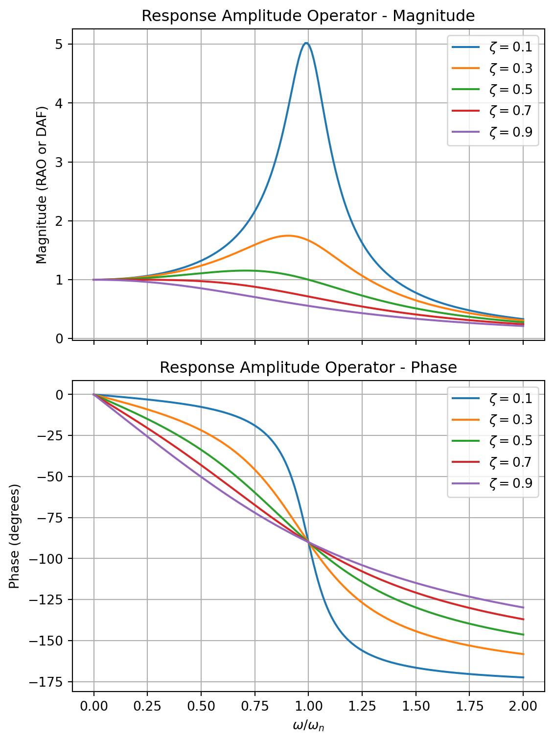
The plot of the RAO for various values of damping ratios is shown in Figure 2.7. We can see that for a low damping ratio, the amplitude of the response amplifies significantly when \(\omega/\omega_n \approx 1\). This phenomenon (\(\omega/\omega_n = 1\)) is known as resonance and in case of undamped system (\(\zeta = 0\)) the response amplitude goes to infinity. When \(\omega/\omega_n \rightarrow 0\), the RAO tends to unity and when \(\omega/\omega_n \rightarrow \infty\), the RAO tends to zero.
For \(\zeta \ll 1\) and \(\omega/\omega_n < 1\), the response tends to be in phase with the excitation. However, for \(\omega/\omega_n > 1\) the response tends to be out of phase (\(-180^\circ\)) with the excitation. For larger damping ratios, this progression is more gradual. For all damping cases, the response phase is \(-90^\circ\) with respect to the excitation at \(\omega/\omega_n = 1\).
The total solution is the combination of the homogeneous solution (free vibration solution) and the particular solution (forced vibration solution) and is given by:
\[\begin{align} x_c(t) = e^{-\zeta \omega_n t} \left(A_h e^{i\omega_dt} + B_h e^{-i\omega_dt}\right) + \frac{f_0/\omega_n^2}{\left(1 - \frac{\omega^2}{\omega_n^2}\right) + i 2 \zeta \frac{\omega}{\omega_n}} e^{i\omega t} \end{align}\]
where \(A_h\) and \(B_h\) are determined from the initial conditions.
Interactive Simulation
Use the tool below to explore how the natural frequency \(\omega_n\), damping ratio \(\zeta\), frequency ratio \(\omega/\omega_n\) and excitation amplitude \(f_0\) affect the forced vibration response of the spring mass damper system. The first plot overlays the excitation \(f(t)/f_0 = \cos(\omega t)\) (right axis) and the non-dimensional response \(x(t)/(f_0/\omega_n^2)\) (left axis) on a common time axis so that the phase difference between them is visible directly. The second plot shows the full RAO curve for the current damping ratio, with a dot marking the current operating point \(\omega/\omega_n\). The third plot shows the phase space trajectory (\(x\) vs. \(\dot{x}\)) of the total response, including the initial transient.
Excitation & Response vs Time
Response Amplitude Operator
Phase Space
2.6 Principle of Superposition
In Section 2.5 we have looked at the response of the single degree of freedom system to a sinusoidal excitation. Let’s see what happens if the excitation is composed to two sinusiods added together. So now we have:
\[\begin{align} F(t) = F_1 \cos(\omega_1 t) + F_2 \sin(\omega_2 t) \end{align}\]
and the corresponding differential equation is given by:
\[\begin{align} m \frac{d^2x}{dt^2} + b \frac{dx}{dt} + kx = F(t) = F_1 \cos(\omega_1 t) + F_2 \sin(\omega_2 t) \end{align}\]
The particular response \(x_1(t)\) for the case \(F(t) = F_1 \cos(\omega_1 t) = \operatorname{Re} \left(F_1 e^{i\omega_1 t}\right)\) is given by:
\[\begin{align} x_1(t) = \operatorname{Re} \left(\frac{F_1/k}{\left(1 - \frac{\omega_1^2}{\omega_n^2}\right) + i 2 \zeta \frac{\omega_1}{\omega_n}} e^{i\omega_1 t}\right) \end{align}\]
Similarly that particular response \(x_2(t)\) for the case \(F(t) = F_2 \sin(\omega_2 t) = \operatorname{Re} \left(F_2 e^{i(\omega_2 t - \frac{\pi}{2})}\right)\) is given by:
\[\begin{align} x_2(t) &= \operatorname{Im} \left(\frac{F_2/k}{\left(1 - \frac{\omega_2^2}{\omega_n^2}\right) + i 2 \zeta \frac{\omega_2}{\omega_n}} e^{i\omega_2 t}\right) \nonumber \\ &= \operatorname{Re} \left(\frac{F_2/k}{\left(1 - \frac{\omega_2^2}{\omega_n^2}\right) + i 2 \zeta \frac{\omega_2}{\omega_n}} e^{i(\omega_2 t - \frac{\pi}{2})}\right) \end{align}\]
It can be seen that the particular solution \(x_p(t) = x_1(t) + x_2(t)\) satisfies the differential equation.
\[\begin{align} m \frac{d^2x_p}{dt^2} + b \frac{dx_p}{dt} + kx_p &= m \frac{d^2x_1}{dt^2} + b \frac{dx_1}{dt} + kx_1 + m \frac{d^2x_2}{dt^2} + b \frac{dx_2}{dt} + kx_2 \nonumber \\ &= F_1 \cos(\omega_1 t) + F_2 \sin(\omega_2 t) \end{align}\]
The steady state response \(x_p(t)\) of the system is equal to the superposition of the steady state responses (\(x_1(t)\) and \(x_2(t)\)) to the individual force components (\(F_1 \cos(\omega_1 t)\) and \(F_2 \sin(\omega_2 t)\)). Hence the name principle of superposition. Note that this principle of superposition is valid only for linear differential equations.
The total solution for this case is given by:
\[\begin{align} x(t) &= x_h(t) + x_p(t) \nonumber \\ &= \operatorname{Re} \left( e^{-\zeta \omega_n t} \left(A_h e^{i\omega_dt} + B_h e^{-i\omega_dt}\right) + \frac{F_1/k}{\left(1 - \frac{\omega_1^2}{\omega_n^2}\right) + i 2 \zeta \frac{\omega_1}{\omega_n}} e^{i\omega_1 t}\right. \nonumber \\ &\qquad \left. + \frac{F_2/k}{\left(1 - \frac{\omega_2^2}{\omega_n^2}\right) + i 2 \zeta \frac{\omega_2}{\omega_n}} e^{i(\omega_2 t - \frac{\pi}{2})}\right) \end{align}\]
where the constants \(A_h\) and \(B_h\) are determined from the initial conditions.
Interactive Simulation
Use the tool below to explore how the force amplitudes \(F_1\), \(F_2\), the forcing frequencies \(\omega_1\), \(\omega_2\), the natural frequency \(\omega_n\), damping ratio \(\zeta\) and the initial conditions \(x_0\), \(v_0\) affect the total response of the system. The first plot shows the total response \(x(t)\) (solid) together with the decaying transient/homogeneous part alone (dashed) so that you can see the response settle into its steady state. The second plot shows the RAO curve for the current damping ratio, with two dots marking the operating points \(\omega_1/\omega_n\) and \(\omega_2/\omega_n\). The third plot shows the phase space trajectory (\(x\) vs. \(\dot{x}\)) of the total response, including the initial transient.
Total Response vs Time
Response Amplitude Operator
Phase Space
2.7 Tutorial: Heave motion of a spar platform
One of the popular designs of an offshore platform is the classic spar platform. The spar is primarily a large cylinder with a very deep draft. Let us consider a spar of diameter \(D\) and a draft of \(T\). Assuming that the spar is floating freely without any mooring lines, the weight of the spar will be equal to the weight of the volume of water displaced (Archimedes’ Principle). Thus the weight of the spar \(W\) is equal to buoyancy \(B\) and is given by:
\[\begin{align} W = B = \rho g \nabla = \rho g \left(\frac{\pi D^2 T}{4}\right) \end{align}\]
Now consider that we move the spar up by a distance \(\Delta \xi_3\) (known as heave displacement). This will result in reduced buoyancy and the net difference between the weight and the reduced buoyancy will result in a net force \(F_{3s}\) given by:
\[\begin{align} F_{3s} = -\frac{\rho g \pi D^2}{4} \Delta \xi_3 \end{align}\]
The negative sign indicates that the force acts in a direction opposite to the displacement \(\Delta \xi_3\). This net restoring force tries to restore the spar back to its static equlibrium position. Thus, it acts very much like a spring with a stiffness of \(C_{33}\):
\[\begin{align} C_{33} = \frac{\rho g \pi D^2}{4} \end{align}\]
The undamped equation of motion for the spar can then be written as:
\[\begin{align} &\rho \nabla \frac{d^2\xi_3}{dt^2} + C_{33} \xi_3 = 0 \nonumber \\ &\frac{d^2\xi_3}{dt^2} + \frac{g}{T} \xi_3 = 0 \end{align}\]
We can compute the natural frequency of the system \(\omega_{n3}\) as:
\[\begin{align} \omega_{n3} = \sqrt{\frac{C_{33}}{\rho \nabla}} = \sqrt{\frac{g}{T}} \end{align}\]
We will later see that this is not quite right as we neglected the added mass of the spar platform in this computation. However, neglecting the effect of added mass for now, we can see that the natural frequency is inversely proportional to the draft of the platform \(T\). If the spar platform experiences a regular wave of frequency \(\omega\), we know from our discussion above that the response amplitude will be governed by ratio \(\omega/\omega_{n3}\). When \(\omega/\omega_{n3} \rightarrow 1\), the platform will experience resonance and the platform will experience a large heave response. Thus during the design process of an offshore structure, it is important to ensure that the dimensions are chosen such that our natural frequency is away from the frequency of waves that the offshore structure might experience at the installation site.
2.8 Exercises
Unless stated otherwise, use \(\rho = 1025\) kg/m\(^3\) and \(g = 9.81\) m/s\(^2\). Every problem below can be solved using only the results derived in this chapter — the free vibration solutions of Section 2.2 and Section 2.4, the RAO of Section 2.5, the principle of superposition, and the hydrostatic restoring argument of the spar tutorial — together with the elementary hydrostatics (\(KB\), \(BM\), \(GM\)) you have already met. In particular the added mass, radiation damping and wave excitation forces on a floating body are not required: wherever a hydrodynamic force acts, its amplitude is given to you directly.
The principal dimensions quoted for real platforms are approximate published figures and are used only to give the numbers a realistic scale. Several problems ask you to derive a result before using it numerically — the derivation carries most of the marks.
The four hull forms used in these exercises
Problems 1, 2, 3 and 9 all concern the same four kinds of floating unit, and it is worth knowing what they look like before working with their numbers. Figure 2.8 shows the four types in service. As you look at each photograph, note how much of the structure actually crosses the waterline and how much of it is hidden below: the four differ enormously in that respect, and Problem 1 asks you to work out what follows from the difference.
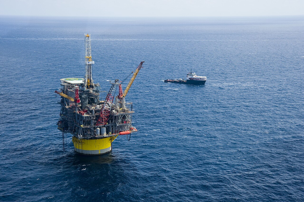
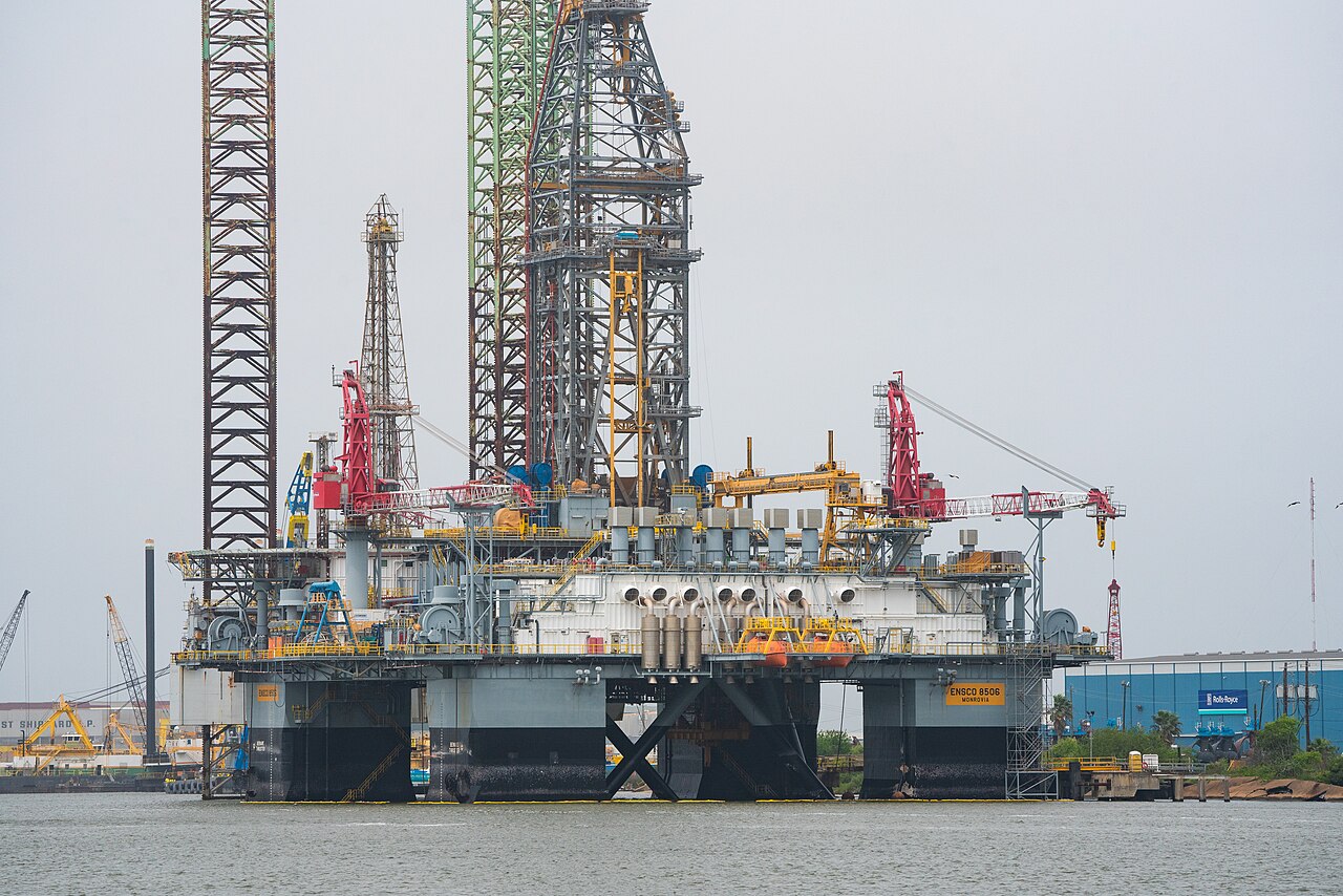
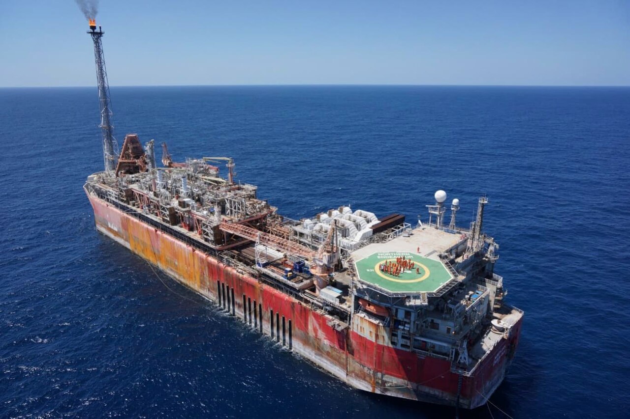
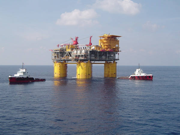
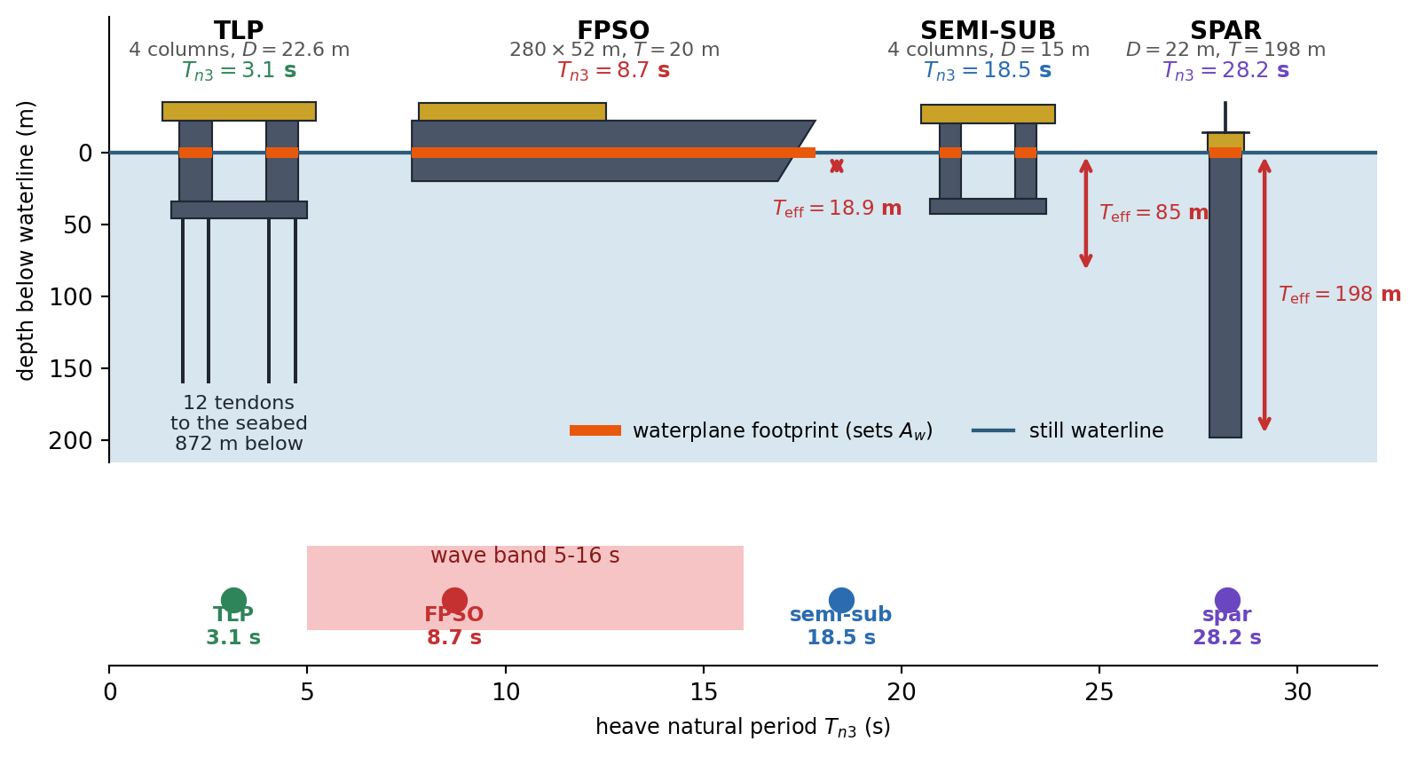
Figure 2.9 redraws the same four units to a common scale from the dimensions quoted in the problems, so that the photographs can be read quantitatively. The orange bar marks the part of each hull that crosses the waterline. Nothing further is annotated, deliberately: what these four shapes imply for the heave motion is the business of Problems 1 and 9, and the same drawing appears again in the answer key with those results added.
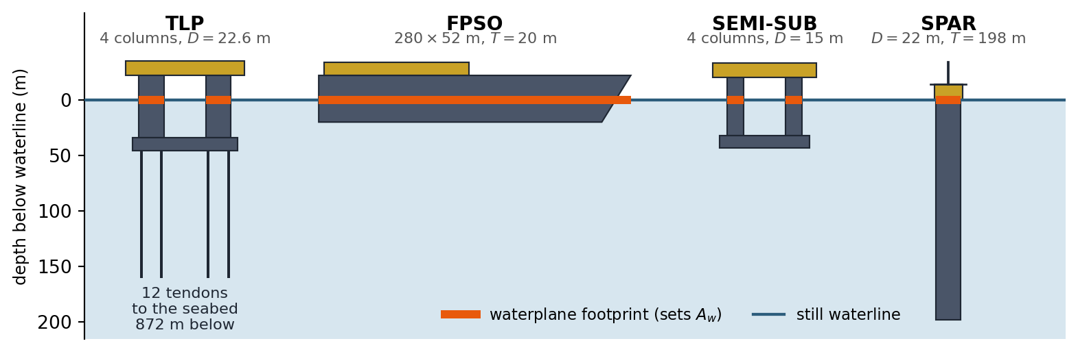
What actually sets the heave natural period. The tutorial derived the heave natural frequency of a vertical circular cylinder. We now generalise it and apply it to four real floating units.
- For a freely floating body of arbitrary shape with waterplane area \(A_w\) (assumed constant over small heave) and displaced volume \(\nabla\), repeat the tutorial’s argument to show that \[\omega_{n3} = \sqrt{\frac{g A_w}{\nabla}} = \sqrt{\frac{g}{T_{\text{eff}}}}, \qquad T_{\text{eff}} = \frac{\nabla}{A_w}\] and verify that \(T_{\text{eff}}\) reduces to the draft for a vertical cylinder. Note carefully that \(\rho\) cancels.
- The Neptune spar (Gulf of Mexico, 1996 — the first production spar) has a hull diameter of \(22\) m and a draft of \(198\) m. The Genesis spar (1998) has a hull diameter of \(37.2\) m and a draft of \(168\) m. Compute \(\nabla\), the displaced mass and the heave natural period of each. Genesis displaces roughly two and a half times as much as Neptune — why are their heave natural periods so similar?
- A column-stabilised semi-submersible has four surface-piercing circular columns of diameter \(15\) m and a total displaced volume (columns plus submerged pontoons) of \(6.0 \times 10^4\) m\(^3\). Compute \(A_w\), \(T_{\text{eff}}\) and the heave natural period.
- An FPSO has \(L = 280\) m, \(B = 52\) m, draft \(20\) m, block coefficient \(C_b = 0.85\) and waterplane coefficient \(C_w = 0.90\). Compute \(\nabla\), \(A_w\), \(T_{\text{eff}}\) and the heave natural period. Compare all four units against a wave band of \(5\)–\(16\) s.
- To what draft would the FPSO have to be loaded, at fixed \(C_b\) and \(C_w\), for its heave natural period to reach \(20\) s? Comment on your answer.
Pitch of a spar, and why a huge \(GM\) is not a problem. Consider the Genesis spar: hull diameter \(D = 37.2\) m, draft \(T = 168\) m, floating freely at even keel. The fixed ballast carried at the keel places the centre of gravity at \(KG = 60\) m above the keel, and the pitch radius of gyration about the centre of gravity is \(k_{55} = 62\) m.
- Compute \(\nabla\), \(KB\), \(BM\) and \(GM\). Comment on the relative size of \(BM\) and \(KB - KG\). How does a spar get its stability, compared with a conventional ship?
- For a small pitch angle \(\xi_5\) the hydrostatic righting moment is \(\rho g \nabla \, GM \, \xi_5\). Write the undamped pitch equation of motion, identify the rotational stiffness \(C_{55}\) and the pitch mass moment of inertia \(I_{55}\), and hence show that \[T_{n5} = 2\pi \frac{k_{55}}{\sqrt{g\,GM}}\] Note that the displacement cancels completely — this is the same result you met in hydrostatics for the roll period of a ship.
- Evaluate \(C_{55}\), \(I_{55}\) and \(T_{n5}\) for Genesis.
- During a modification, ballast is transferred from the keel to the topsides so that \(KG\) rises to \(72\) m at unchanged displacement and unchanged \(k_{55}\). Compute the new \(GM\) and \(T_{n5}\). Does raising \(KG\) move the spar towards or away from the wave band?
- At what \(KG\) would the spar become neutrally stable? Separately, what \(GM\) (and hence what \(KG\)) would be needed to bring \(T_{n5}\) down to \(16\) s? Comment on whether a spar can be made to resonate in pitch with ordinary waves.
- An FPSO has \(GM = 4.5\) m and a roll radius of gyration \(k_{44} = 18.2\) m. Compute its roll natural period. The spar has a \(GM\) more than five times larger, yet a longer natural period. Explain. Then state one reason your computed spar period is an underestimate of the real one.
A pitch free-decay test on the Neptune spar. The Neptune spar has a hull diameter of \(22\) m, a draft of \(198\) m and \(KG = 78\) m. In a model-scale free-decay test (results given at full scale) the platform is heeled over in pitch and released. The first positive peak is \(4.00^\circ\), the sixth positive peak is \(1.28^\circ\), and the two peaks are \(235\) s apart.
- Starting from the underdamped free-vibration solution, show that the ratio of two positive peaks \(n\) cycles apart is \(\exp\left(2\pi n\zeta/\sqrt{1-\zeta^2}\right)\), and hence determine \(\zeta\). Explain why working in degrees rather than radians does not affect the answer.
- Determine \(T_d\), \(\omega_d\), \(\omega_{n5}\) and \(T_{n5}\).
- Compute \(\nabla\), \(GM\) and the pitch restoring stiffness \(C_{55}\). Combining this with the measured natural frequency, determine the apparent pitch moment of inertia \(I_{55}\), the corresponding apparent radius of gyration, and the pitch damping coefficient \(b_{55}\).
- The structural designer’s estimate of the pitch radius of gyration is \(65\) m. Compute the natural period this predicts and compare it with the measured value. By what factor does the apparent inertia exceed the structural inertia? What physics, deliberately left out of this chapter, accounts for the difference?
- How many complete cycles are needed for the pitch amplitude to fall below \(5\%\) of its initial value? Would the answer change if the platform had been heeled to \(8^\circ\) instead of \(4^\circ\)? Justify from the governing equation.
Sizing a berthing fender. An LNG carrier of effective mass \(1.2 \times 10^8\) kg approaches a berth and strikes a fender of stiffness \(k = 5.0 \times 10^6\) N/m with a normal approach speed of \(0.15\) m/s. Model the vessel–fender system as a single degree of freedom system with \(x(0) = 0\) and \(\dot{x}(0) = v_0\), and idealise the fender as a linear spring and dashpot that remain in contact with the hull throughout.
- Compute \(\omega_n\) and \(T_n\).
- For an undamped fender (\(\zeta = 0\)), find the maximum compression, the maximum fender force, and describe what the vessel does afterwards.
- For a critically damped fender (\(\zeta = 1\)), show that \(x(t) = v_0 t e^{-\omega_n t}\), and hence that the maximum compression is \(v_0/(e\,\omega_n)\) occurring at \(t = 1/\omega_n\). Show also that the vessel never rebounds.
- For an overdamped fender (\(\zeta = 2\)), find the maximum compression and the time at which it occurs.
- The total force transmitted by the fender is \(F(t) = kx + b\dot{x}\). For the critically damped case, show that \(F\) is largest at the instant of impact and equals \(bv_0 = 2m\omega_n v_0\), exactly twice the undamped peak force. Evaluate the peak force for \(\zeta = 1\) and \(\zeta = 2\) and discuss the trade-off a fender designer faces between stroke and peak load.
Where is the resonant peak, really?
- Starting from \(|H(\omega)|\), show that the RAO magnitude is a maximum at \(r = \omega/\omega_n = \sqrt{1-2\zeta^2}\) with peak value \(1/\left(2\zeta\sqrt{1-\zeta^2}\right)\), and that such a peak exists only if \(\zeta < 1/\sqrt{2}\).
- For a moored structure with \(\omega_n = 0.35\) rad/s and \(\zeta = 0.08\), compute the wave frequency and wave period producing the largest response, the peak RAO, and compare both with the values at \(\omega = \omega_n\).
- Repeat for \(\zeta = 0.5\) and for \(\zeta = 0.75\), and describe qualitatively how the RAO curve changes.
- A classmate states: “the largest response always occurs when the wave frequency equals the natural frequency.” Is this correct? When is it a safe engineering approximation, and when does it fail outright?
The forces you do not see. The sway of the deck of a fixed jacket platform is modelled as a single degree of freedom system with \(m = 8.0 \times 10^6\) kg, natural period \(T_n = 4.0\) s and \(\zeta = 0.03\). A wave train of period \(4.0\) s produces a horizontal force of amplitude \(F_0 = 2.0\) MN.
- Compute \(k\) and \(b\).
- Compute the steady-state deck amplitude and its phase relative to the wave force.
- Compute the amplitudes of the inertia force \(m\omega^2|A_c|\), the damping force \(b\omega|A_c|\) and the elastic force \(k|A_c|\). Show that the inertia and elastic forces cancel exactly and that the entire wave force is resisted by the dashpot alone.
- By what factor do the internal elastic forces exceed the applied wave force? Express this factor in terms of \(\zeta\) alone and comment on the structural consequence.
- The designer stiffens the jacket, keeping the mass and damping ratio unchanged, so that the RAO at a wave period of \(4.0\) s is at most \(1.25\). Find the required natural period, the required stiffness and the resulting deck amplitude. What design philosophy for bottom-founded structures does this illustrate?
A small force in exactly the wrong place. A moored floating structure has \(m = 3.0 \times 10^7\) kg, \(\omega_n = 0.25\) rad/s and \(\zeta = 0.05\). It is excited by \[F(t) = F_1\cos(\omega_1 t) + F_2\sin(\omega_2 t)\] with \(F_1 = 4.0\) MN at \(\omega_1 = 0.60\) rad/s (locally generated wind sea) and \(F_2 = 0.5\) MN at \(\omega_2 = 0.26\) rad/s (a distant swell).
- Compute the steady-state amplitude and phase of each response component.
- The swell force is eight times smaller than the wind-sea force. What is the ratio of the two response amplitudes? Explain the physical reason in one sentence.
- Write down an upper bound for \(|x(t)|\) and state the condition under which it is attained. Is it attained here?
- A consultant proposes tripling the damping to \(\zeta = 0.15\) by fitting damping devices. Recompute both components and comment on which one benefits, and by how much. What general rule about damping does this illustrate?
How long does resonance take to build up? A moored structure with \(\omega_n = 0.30\) rad/s and \(\zeta = 0.02\) is initially at rest (\(x_0 = 0\), \(v_0 = 0\)). At \(t = 0\) a regular wave train at exactly \(\omega = \omega_n\) begins to act, with a static deflection \(F_0/k = 0.05\) m.
- Write the total solution satisfying the initial conditions and show that for \(\zeta \ll 1\) the response is approximately \(X\left(1 - e^{-\zeta\omega_n t}\right)\sin(\omega_n t)\), where \(X\) is the steady-state amplitude.
- Compute \(X\).
- Compute the time and the number of cycles required for the envelope to reach \(95\%\) of \(X\).
- Show that the number of cycles to reach \(95\%\) of steady state is \(N_{95} = \ln(20)/(2\pi\zeta)\), independent of \(\omega_n\) and of the force amplitude.
- Swell at the site arrives in groups of about \(8\) well-formed waves before the phase breaks down. What fraction of the steady-state amplitude is actually reached? What does this tell you about applying steady-state RAO results to a real, irregular sea? Contrast with the spar pitch mode of Problem 3.
Two opposite ways of escaping the waves. Compare two units at the same site. Take \(\zeta = 0.05\) in heave and a heave excitation force amplitude of \(1.0\) MN for both.
- TLP (dimensions typical of the Auger TLP, Gulf of Mexico, \(872\) m water depth): held down by twelve vertical steel tendons, each of Young’s modulus \(E = 2.1 \times 10^{11}\) Pa, cross-sectional area \(A = 0.060\) m\(^2\) and length \(L = 872\) m, so that each contributes an axial stiffness \(EA/L\). The hull has four surface-piercing columns of diameter \(22.6\) m, and the effective heave mass is \(4.7 \times 10^7\) kg. The tendon and hydrostatic stiffnesses act in parallel and therefore add.
- Spar: the Neptune spar of Problem 1 (\(D = 22\) m, \(T = 198\) m).
- Compute the TLP heave stiffness, the percentage contributed by the tendons, and its \(\omega_n\) and \(T_n\).
- State the spar’s heave \(\omega_n\) and \(T_n\).
- For a wave period of \(12\) s, compute \(r\), the RAO and the heave amplitude of each unit. For each, state which of the three terms in the equation of motion (stiffness, damping, inertia) dominates.
- A long swell of period \(28\) s now arrives. Repeat and comment.
- Both hulls avoid resonance in the \(5\)–\(16\) s band, but by opposite strategies. Describe them, and use your numbers to explain why “a small RAO means small motion” and “an RAO near unity means large motion” are both false statements.
Programming Problem: The structure as a filter. A moored floating structure has \(m = 4.0\times10^7\) kg, \(\omega_n = 0.28\) rad/s and \(\zeta = 0.06\). The sea state produces a heave excitation force made up of six harmonic components, \[F(t) = \sum_{j=1}^{6} F_j\cos\left(\omega_j t + \varepsilon_j\right)\]
\(j\) 1 2 3 4 5 6 \(\omega_j\) (rad/s) 0.20 0.28 0.40 0.55 0.70 0.90 \(F_j\) (MN) 0.8 0.4 1.5 2.5 1.8 0.9 \(\varepsilon_j\) (deg) 0 45 120 200 310 75 - Compute \(k\), and for each component the frequency ratio, the RAO magnitude and phase, and the steady-state response amplitude.
- Which component carries the largest force? Which produces the largest motion? Tabulate the percentage each component contributes to \(\sum_j F_j\) and to \(\sum_j |x_j|\).
- Construct \(x(t)\) over \(0 \le t \le 1200\) s and find \(\max|x(t)|\). Compare with the bound \(\sum_j |x_j|\).
- Explain, using your table from (b), in what sense the structure acts as a filter on the sea, and why a component carrying only about \(5\%\) of the total force amplitude produces more than \(40\%\) of the motion.
- Investigate three proposed fixes and report the resulting \(\sum_j|x_j|\) for each: (i) fitting damping devices that raise \(\zeta\) to \(0.18\); (ii) stiffening the mooring so that \(k\) is multiplied by \(2\), by \(4\) and by \(16\) (the mass being unchanged); (iii) halving the largest force component \(F_4\). Which of them actually work? Explain the behaviour of (ii) in particular — the answer is not monotonic, and the reason is the whole point of the problem.
Answer Key
Problem 1 — What actually sets the heave natural period
- (a) Raising the body by \(\Delta\xi_3\) removes a slice of buoyancy of volume \(A_w\Delta\xi_3\), so \(F_{3s} = -\rho g A_w \Delta\xi_3\) and \(C_{33} = \rho g A_w\). With mass \(\rho\nabla\), \(\omega_{n3} = \sqrt{C_{33}/(\rho\nabla)} = \sqrt{gA_w/\nabla}\); \(\rho\) cancels, so the natural period is a purely geometric property of the hull. For a cylinder \(\nabla = A_w T\), giving \(T_{\text{eff}} = T\).
- (b) Neptune: \(\nabla = 75266\) m\(^3\), mass \(= 77.1\) kt, \(T_{n3} = 28.23\) s. Genesis: \(\nabla = 182593\) m\(^3\), mass \(= 187.2\) kt, \(T_{n3} = 26.00\) s. For a cylinder \(T_{\text{eff}}\) is the draft, so \(T_{n3} = 2\pi\sqrt{T/g}\) depends on the draft alone — the diameter cancels between stiffness and mass. Genesis is much larger in every other respect, but its draft is only \(15\%\) less, so its heave period is only \(8\%\) shorter. Displacement is not the design lever; the ratio \(\nabla/A_w\) is.
- (c) \(A_w = 4\times\pi(15)^2/4 = 706.9\) m\(^2\), \(T_{\text{eff}} = 84.88\) m, \(T_{n3} = 18.48\) s. The semi hides almost all of its buoyancy below the free surface and pierces it with slender columns, buying a long heave period at a draft of only a few tens of metres.
- (d) FPSO: \(\nabla = 247520\) m\(^3\) (mass \(253.7\) kt), \(A_w = 13104\) m\(^2\), \(T_{\text{eff}} = C_bT/C_w = 18.89\) m, \(T_{n3} = 8.72\) s. Summary: Neptune \(28.2\) s and Genesis \(26.0\) s sit safely above the band; the semi at \(18.5\) s is just above it; the FPSO at \(8.7\) s sits squarely inside it and will heave strongly — which is why FPSOs are chosen for their storage and offloading capability rather than for their motions.
- (e) Need \(T_{\text{eff}} = g(20/2\pi)^2 = 99.4\) m, i.e. a draft of \(T = C_wT_{\text{eff}}/C_b = 105\) m. This is absurd — five times the depth of the hull. A ship-shaped hull cannot be taken out of the wave band in heave by loading it; escaping the band requires a fundamentally different hull form (spar, semi) or a fundamentally different restoring mechanism (TLP tendons, Problem 9).
Problem 2 — Pitch of a spar, and why a huge \(GM\) is not a problem
- (a) \(\nabla = 182593\) m\(^3\), \(KB = T/2 = 84.0\) m, \(I_{wp} = \pi D^4/64 = 94003\) m\(^4\), \(BM = I_{wp}/\nabla = 0.5148\) m, \(GM = KB + BM - KG = 24.515\) m. \(BM\) contributes only \(2.1\%\) of \(GM\): for a deep slender cylinder \(BM = D^2/(16T)\) is tiny. A spar is stable because its centre of gravity is held below its centre of buoyancy (\(KG < KB\)), like a weighted pendulum, whereas a ship has \(KG > KB\) and relies almost entirely on the large \(BM\) of its wide waterplane.
- (b) \(I_{55}\ddot{\xi}_5 + C_{55}\xi_5 = 0\) with \(C_{55} = \rho g \nabla\, GM\) and \(I_{55} = \rho\nabla k_{55}^2\). Hence \[\omega_{n5}^2 = \frac{C_{55}}{I_{55}} = \frac{\rho g\nabla\,GM}{\rho\nabla k_{55}^2} = \frac{g\,GM}{k_{55}^2} \quad\Longrightarrow\quad T_{n5} = \frac{2\pi k_{55}}{\sqrt{g\,GM}}\] The displacement cancels exactly as it did in heave. Only two numbers matter: the metacentric height and the radius of gyration.
- (c) \(C_{55} = 4.5010 \times 10^{10}\) N·m/rad, \(I_{55} = 7.1944 \times 10^{11}\) kg·m\(^2\), \(\omega_{n5} = 0.2501\) rad/s, \(T_{n5} = 25.12\) s — comfortably above the wave band.
- (d) \(GM = 12.515\) m and \(T_{n5} = 35.16\) s. Since \(T_{n5} \propto 1/\sqrt{GM}\), raising \(KG\) lengthens the period by \(\sqrt{24.51/12.51} = 1.400\) and therefore moves the spar further away from the wave band. A larger \(GM\) is not automatically better: it stiffens the restoring and shortens the period, pulling the natural period down towards the waves.
- (e) Neutral stability at \(GM = 0\), i.e. \(KG = KB + BM = 84.51\) m; as \(GM \to 0\) the restoring vanishes and \(T_{n5} \to \infty\). For \(T_{n5} = 16\) s we would need \(GM = g^{-1}(2\pi k_{55}/16)^2 = 60.4\) m, i.e. \(KG = 24.1\) m — the whole mass of the platform concentrated within \(24\) m of the keel of a \(168\) m draft hull. Physically unreachable: a spar cannot be made to resonate in pitch with ordinary wind waves. Its slow pitch mode is instead excited by swell, wave groups and wind.
- (f) FPSO roll: \(T_{n4} = 2\pi k_{44}/\sqrt{g\,GM} = 17.21\) s — at the top of the wave band, the classic roll-resonance problem. The spar has \(GM = 24.5\) m against the FPSO’s \(4.5\) m, a factor \(5.45\), but its radius of gyration is \(3.41\) times larger, and the period depends on \(k/\sqrt{GM}\): \(3.41/\sqrt{5.45} = 1.46\), so the spar period is longer by that factor (\(25.1\) s vs \(17.2\) s). Inertia beats stiffness here. Finally, the computed spar period is an underestimate because the pitch added moment of inertia of the water entrained by a \(168\) m deep hull — neglected throughout this chapter, exactly as the tutorial warned for heave — is comparable to or larger than the structural \(I_{55}\). Problem 3 measures how large it actually is.
Problem 3 — A pitch free-decay test on the Neptune spar
- (a) With \(\xi_5(t) = e^{-\zeta\omega_n t}(A\cos\omega_d t + B\sin\omega_d t)\), successive positive peaks are exactly \(T_d = 2\pi/\omega_d\) apart and the bracket repeats, so \(\xi_i/\xi_{i+n} = e^{\zeta\omega_n nT_d} = \exp\left(2\pi n\zeta/\sqrt{1-\zeta^2}\right)\). Hence \(\delta = \frac{1}{5}\ln(4.00/1.28) = 0.22789\) and \(\zeta = \delta/\sqrt{4\pi^2+\delta^2} = 0.03625\) (\(3.62\%\)). Degrees are fine because only the ratio of two amplitudes enters, and the unit cancels — a consequence of the equation being linear and homogeneous.
- (b) \(T_d = 235/5 = 47.0\) s, \(\omega_d = 0.13368\) rad/s, \(\omega_{n5} = \omega_d/\sqrt{1-\zeta^2} = 0.13377\) rad/s, \(T_{n5} = 46.97\) s.
- (c) \(\nabla = 75266\) m\(^3\), \(KB = 99.0\) m, \(BM = 0.1528\) m, \(GM = 21.153\) m, \(C_{55} = \rho g\nabla\,GM = 1.6009 \times 10^{10}\) N·m/rad. From \(I_{55} = C_{55}/\omega_{n5}^2\) we get \(I_{55} = 8.9459 \times 10^{11}\) kg·m\(^2\), i.e. an apparent radius of gyration \(k = \sqrt{I_{55}/(\rho\nabla)} = 107.7\) m. \(b_{55} = 2\zeta\sqrt{I_{55}C_{55}} = 8.6752 \times 10^{9}\) N·m·s/rad.
- (d) With \(k_{55} = 65\) m, \(I_{55}^{struct} = 3.2595 \times 10^{11}\) kg·m\(^2\) and \(T_{n5} = 2\pi\sqrt{I/C_{55}} = 28.35\) s, against a measured \(46.97\) s. The apparent inertia exceeds the structural inertia by a factor \((47.0/28.4)^2 = 2.74\). Note also that the apparent radius of gyration, \(108\) m, is larger than half the draft — no distribution of the platform’s own steel and ballast could produce it. The missing physics is the added moment of inertia of the water entrained by the deep hull as it pitches — precisely the added-mass effect the tutorial flagged as neglected. Here it contributes about \(64\%\) of the total effective inertia (with a smaller contribution from the mooring system). This is why a spar’s measured pitch period is far longer than a dry-structure calculation suggests, and why the next chapters must put added mass back in.
- (e) \(N = \ln(20)/\delta = 13.15\), so 14 complete cycles. The answer is unchanged for an initial heel of \(8^\circ\): the equation of motion is linear and homogeneous, so doubling the initial condition doubles the entire record and leaves every amplitude ratio — and hence \(\zeta\), \(T_d\) and \(N\) — untouched. (Real spar pitch damping is partly viscous and therefore amplitude-dependent, so a real decay test would show a small drift in \(\delta\) from cycle to cycle; a constant \(\delta\) is itself evidence that the linear model is adequate.)
Problem 4 — Sizing a berthing fender
- (a) \(\omega_n = \sqrt{k/m} = 0.20412\) rad/s, \(T_n = 30.78\) s.
- (b) \(x = (v_0/\omega_n)\sin\omega_n t\), so \(x_{max} = 0.7348\) m at \(t = T_n/4 = 7.70\) s and \(F_{max} = kx_{max} = 3.67\) MN. The vessel then rebounds off the berth with the full approach speed of \(0.15\) m/s — all the kinetic energy is handed straight back, which is exactly what a fender must not do.
- (c) For \(\zeta = 1\), \(x = (A+Bt)e^{-\omega_n t}\); \(x(0)=0\Rightarrow A=0\), \(\dot{x}(0)=B=v_0\). Then \(\dot{x} = v_0(1-\omega_n t)e^{-\omega_n t} = 0\) gives \(t = 1/\omega_n = 4.90\) s and \(x_{max} = v_0/(e\omega_n) = 0.2703\) m, only \(1/e = 0.368\) of the undamped stroke. Since \(te^{-\omega_n t} > 0\) for all \(t > 0\), \(x\) never returns through zero: the vessel creeps back without rebounding.
- (d) For \(\zeta = 2\), \(s_{1,2} = -\omega_n(\zeta \mp \sqrt{\zeta^2-1}) = -0.05469,\ -0.76180\) s\(^{-1}\), \(x = C(e^{s_1t}-e^{s_2t})\) with \(C = v_0/(s_1-s_2) = 0.21213\) m. \(\dot{x}=0\) gives \(t^* = \ln(s_2/s_1)/(s_1-s_2) = 3.72\) s and \(x_{max} = 0.1606\) m.
- (e) For \(\zeta = 1\), \(b\omega_n = 2m\omega_n^2 = 2k\), so \(F = v_0e^{-\omega_nt}[kt + b(1-\omega_nt)] = v_0e^{-\omega_nt}(b-kt)\), which is largest at \(t = 0\) with \(F(0) = bv_0 = 2m\omega_nv_0 = 2(kv_0/\omega_n)\) — twice the undamped peak. Numerically \(F_{max} = 7.35\) MN for \(\zeta = 1\) and \(14.70\) MN for \(\zeta = 2\), against \(3.67\) MN undamped. The trade-off: damping shrinks the stroke (\(0.735 \to 0.270 \to 0.161\) m) and kills the rebound, but the dashpot force is proportional to velocity and the velocity is greatest at first contact, so the peak load delivered to the berth structure rises with damping. A fender cannot be designed on stroke alone.
Problem 5 — Where is the resonant peak, really?
- (a) \(|H|^{-2} = (1-r^2)^2 + (2\zeta r)^2\). Differentiating with respect to \(r^2\) and setting to zero, \(-2(1-r^2) + 4\zeta^2 = 0 \Rightarrow r_{peak}^2 = 1 - 2\zeta^2\); substituting back, \(|H|_{max} = 1/\left(2\zeta\sqrt{1-\zeta^2}\right)\). A real \(r_{peak} > 0\) requires \(1 - 2\zeta^2 > 0\), i.e. \(\zeta < 1/\sqrt{2} = 0.707\).
- (b) \(r_{peak} = 0.99358\), \(\omega_{peak} = 0.34775\) rad/s, \(T_{peak} = 18.07\) s against \(T_n = 17.95\) s; \(|H|_{max} = 6.2701\) against \(|H(\omega_n)| = 1/(2\zeta) = 6.2500\) — a difference of \(0.32\%\) in amplitude and \(0.64\%\) in frequency.
- (c) \(\zeta = 0.5\): \(r_{peak} = 0.70711\), \(|H|_{max} = 1.1547\) against \(|H(\omega_n)| = 1.000\) — the peak has moved well below \(\omega_n\) and has nearly flattened out. \(\zeta = 0.75 > 1/\sqrt{2}\): no interior peak at all; \(|H|\) falls monotonically from \(|H(0)| = 1\), so the largest response is the quasi-static one and the structure never amplifies anything.
- (d) Strictly incorrect: the displacement RAO peaks slightly below \(\omega_n\), and for \(\zeta \ge 1/\sqrt{2}\) there is no peak whatsoever. It is a safe approximation for lightly damped structures (\(\zeta \lesssim 0.1\)), where the frequency shift is \(O(\zeta^2)\) and the amplitude error is well under \(1\%\) — which is why offshore practice speaks freely of ‘resonance at \(\omega_n\)’. It fails for heavily damped systems and for any mode deliberately fitted with damping devices.
Problem 6 — The forces you do not see
- (a) \(\omega_n = 2\pi/4 = 1.57080\) rad/s, \(k = m\omega_n^2 = 1.9739 \times 10^{7}\) N/m, \(b = 2\zeta\sqrt{mk} = 7.5398 \times 10^{5}\) N·s/m.
- (b) \(\omega = \omega_n\), so \(r = 1\) and \(H = 1/(i2\zeta)\). Static deflection \(F_0/k = 0.10132\) m, amplitude \(|A_c| = (F_0/k)/(2\zeta) = 1.689\) m, phase \(-90^\circ\) — the deck lags the force by a quarter period, so the deck velocity is exactly in phase with the force.
- (c) Inertia \(= m\omega_n^2|A_c| = 33.33\) MN; elastic \(= k|A_c| = 33.33\) MN; damping \(= b\omega_n|A_c| = 2.00\) MN. Since \(m\omega_n^2 = k\), the inertia and elastic forces are equal in magnitude and opposite in phase (displacement and acceleration are \(180^\circ\) apart), so they cancel identically. What is left is \(b\omega_n|A_c| = 2\zeta k\cdot(F_0/k)/(2\zeta) = F_0\). At resonance the excitation is held up by damping alone — which is exactly why the undamped response is unbounded.
- (d) Ratio \(= k|A_c|/F_0 = 1/(2\zeta) = 16.67\). The members carry more than sixteen times the applied wave force and the deck sways \(\pm1.69\) m — both far beyond what a jacket can tolerate. A resonant structure fails not because the sea pushes hard, but because it amplifies a modest push into enormous internal loads.
- (e) Require \((1-r^2)^2 + (2\zeta r)^2 = 1/1.25^2\); with \(u = r^2\), \(u^2 - (2-4\zeta^2)u + (1 - 1/1.25^2) = 0\), whose relevant root is \(u = 0.20045\), \(r = 0.4477\). Hence \(\omega_n \ge \omega/r = 3.508\) rad/s, i.e. \(T_n \le 1.79\) s, requiring \(k \ge 9.8474 \times 10^{7}\) N/m — about \(5\) times stiffer. The deck amplitude falls to \(1.25F_0/k_{new} = 25\) mm. Philosophy: a bottom-founded structure is made stiff, with its natural period pushed well below the wave band, so that it responds quasi-statically (\(r \ll 1\), \(|H| \to 1\)) and the large stiffness itself keeps the motion small. Compliant floating structures do the exact opposite — see Problem 9.
Problem 7 — A small force in exactly the wrong place
- (a) \(k = m\omega_n^2 = 1.8750 \times 10^{6}\) N/m. Wind sea: \(r_1 = 2.40\), \(|H_1| = 0.2098\), \(F_1/k = 2.1333\) m, amplitude \(0.4476\) m at \(-177.1^\circ\). Swell: \(r_2 = 1.04\), \(|H_2| = 7.5648\), \(F_2/k = 0.2667\) m, amplitude \(2.0173\) m at \(-128.1^\circ\). (The \(\sin\) component simply carries an extra \(-90^\circ\): \(x_2 = |H_2|(F_2/k)\cos(\omega_2t - \pi/2 + \phi_2)\).)
- (b) The swell response is \(4.51\) times larger than the wind-sea response despite its force being \(8\) times smaller — a net swing of a factor of \(36\). The reason: \(\omega_2\) sits at \(r_2 = 1.04\), essentially on resonance where \(|H|\approx 1/(2\zeta)\), whereas \(\omega_1\) sits at \(r_1 = 2.4\) deep in the inertia-dominated tail where \(|H| \approx 1/(r^2-1) \ll 1\). Response amplitudes are not in the ratio of the force amplitudes — the RAO reweights them completely.
- (c) By superposition and the triangle inequality, \(|x(t)| \le |x_1| + |x_2| = 2.4649\) m, attained only when both components peak together. Here \(\omega_1/\omega_2 = 30/13\) is rational, so the excitation repeats with period \(2\pi\times13/\omega_1 = 136\) s and the peaks do come into near-alignment: numerically the largest \(|x|\) is \(2.4637\) m, within \(0.05\%\) of the bound. For incommensurate frequencies the bound is approached but never exactly reached.
- (d) With \(\zeta = 0.15\): wind sea \(0.4476 \to 0.4431\) m (a change of only \(1.0\%\)), swell \(2.0173 \to 0.8269\) m (a reduction by a factor of \(2.44\)). Damping only matters near resonance. Away from \(r = 1\) the response is controlled by the stiffness term (\(r \ll 1\)) or the inertia term (\(r \gg 1\)), and the \(2\zeta r\) term is negligible in the denominator of \(H\). Damping devices — heave plates, strakes, bilge keels — earn their cost only for a mode the sea can actually reach.
Problem 8 — How long does resonance take to build up?
- (a) At \(r = 1\) the particular solution is \(x_p = X\sin(\omega_nt)\) with \(X = (F_0/k)/(2\zeta)\) (amplitude \(|H|F_0/k\), phase \(-90^\circ\)). Adding \(x_h = e^{-\zeta\omega_nt}(A\cos\omega_dt + B\sin\omega_dt)\) and imposing \(x(0) = \dot{x}(0) = 0\) gives \(A = 0\) and \(B = -X\omega_n/\omega_d\), so \[x(t) = X\left[\sin(\omega_nt) - \frac{\omega_n}{\omega_d}e^{-\zeta\omega_nt}\sin(\omega_dt)\right]\] For \(\zeta \ll 1\), \(\omega_d \approx \omega_n\) (here \(0.29994\) vs \(0.30000\) rad/s) and the two sines merge, leaving the envelope \(X\left(1 - e^{-\zeta\omega_nt}\right)\).
- (b) \(X = 0.050/(2\times0.02) = 1.250\) m.
- (c) \(1 - e^{-\zeta\omega_nt} = 0.95 \Rightarrow \zeta\omega_nt = \ln 20 = 2.9957\), so \(t_{95} = 499\) s. With \(T_n = 20.94\) s this is \(N = 23.8\) cycles — about 24 waves, over eight minutes of perfectly regular sea.
- (d) \(t_{95} = \ln(20)/(\zeta\omega_n)\) and \(T_n = 2\pi/\omega_n\), so \(N_{95} = t_{95}/T_n = \ln(20)/(2\pi\zeta) = 23.8\). Both \(\omega_n\) and \(F_0\) cancel: build-up is counted in cycles, and the count is set by the damping ratio alone, roughly \(0.48/\zeta\).
- (e) After \(8\) cycles \(\zeta\omega_nt = 2\pi\zeta N = 1.005\), so the envelope has reached \(0.634\), i.e. only about \(63\%\) of \(X\). The steady-state RAO is an upper bound that a real sea — which never holds one frequency and phase for two dozen cycles — may never deliver. The contrast with Problem 3 is instructive: that spar had \(\zeta \approx 3.6\%\) in pitch, giving \(N_{95} \approx 13\) cycles, but a pitch period of \(47\) s, so full build-up would need roughly ten minutes of coherent \(47\) s forcing. A very lightly damped mode (\(\zeta = 0.005\), \(N_{95} \approx 95\) cycles) is effectively protected from short wave groups — but is dangerously exposed to long, regular swell.
Problem 9 — Two opposite ways of escaping the waves
- (a) Tendons: \(12EA/L = 1.7339 \times 10^{8}\) N/m. Hydrostatic: \(A_w = 1605\) m\(^2\), \(\rho gA_w = 1.6135 \times 10^{7}\) N/m. Total \(k = 1.8953 \times 10^{8}\) N/m, of which the tendons supply \(91.5\%\). \(\omega_n = 2.008\) rad/s, \(T_n = 3.13\) s.
- (b) Spar: \(C_{33} = \rho g\pi D^2/4 = 3.8223 \times 10^{6}\) N/m, \(\omega_n = \sqrt{g/T} = 0.2226\) rad/s, \(T_n = 28.23\) s.
- (c) At \(T_w = 12\) s (\(\omega = 0.5236\) rad/s): TLP \(r = 0.2607\), \(|H| = 1.0725\), heave \(= 5.7\) mm — stiffness dominated (\(r \ll 1\)), the tendons take the load quasi-statically. Spar \(r = 2.3523\), \(|H| = 0.2203\), heave \(= 58\) mm — inertia dominated (\(r \gg 1\)), the hull is simply too massive to follow the wave.
- (d) At \(T_w = 28\) s: TLP \(r = 0.1117\), \(|H| = 1.0126\), heave \(= 5.3\) mm — essentially unchanged, because no ocean wave can reach a \(3\) s natural period. Spar \(r = 1.0081\), \(|H| = 9.791\), heave \(= 2.56\) m — the spar is now on resonance and heaves metres from a force that moved it 58 mm at \(12\) s. Deep draft protects a spar from wind sea but places it directly in the path of long swell, which is precisely why real spars carry helical strakes and heave plates to raise \(\zeta\) (and why the \(47\) s pitch mode of Problem 3 matters).
- (e) The TLP escapes upward in frequency: it is made so stiff that \(\omega_n\) lies above the wave band, so \(r \ll 1\) and \(|H| \to 1\). The spar escapes downward in frequency: it is made so compliant and so heavy that \(\omega_n\) lies below the band, so \(r \gg 1\) and \(|H| \to 0\). Both quoted statements are false because the RAO is a ratio, not a motion: at \(12\) s the TLP has \(|H| = 1.07 \approx 1\) yet moves only \(5.7\) mm, because its static deflection \(F_0/k\) is minute; the spar has \(|H| = 0.22 < 1\) yet moves \(58\) mm, ten times more, because its \(F_0/k\) is far larger. Motion is \(|H| \times F_0/k\) — the static deflection must always be carried along with the RAO.
Problem 10 — The structure as a filter
- (a) \(k = m\omega_n^2 = 3.1360 \times 10^{6}\) N/m.
| \(j\) | \(\omega_j\) | \(r_j\) | \(F_j/k\) (m) | \(\lvert H_j\rvert\) | \(\phi_j\) (deg) | \(\lvert x_j\rvert\) (m) |
|---|---|---|---|---|---|---|
| 1 | 0.20 | 0.7143 | 0.2551 | 2.0111 | -9.9 | 0.5130 |
| 2 | 0.28 | 1.0000 | 0.1276 | 8.3333 | -90.0 | 1.0629 |
| 3 | 0.40 | 1.4286 | 0.4783 | 0.9480 | -170.6 | 0.4534 |
| 4 | 0.55 | 1.9643 | 0.7972 | 0.3487 | -175.3 | 0.2779 |
| 5 | 0.70 | 2.5000 | 0.5740 | 0.1902 | -176.7 | 0.1092 |
| 6 | 0.90 | 3.2143 | 0.2870 | 0.1071 | -177.6 | 0.0307 |
- (b) The largest force is component \(4\) (\(\omega = 0.55\) rad/s, \(2.5\) MN), but the largest motion comes from component \(2\) (\(\omega = 0.28\) rad/s \(= \omega_n\), only \(0.4\) MN).
| \(j\) | 1 | 2 | 3 | 4 | 5 | 6 |
|---|---|---|---|---|---|---|
| share of \(\sum F_j\) (%) | 10.1 | 5.1 | 19.0 | 31.6 | 22.8 | 11.4 |
| share of \(\sum \lvert x_j\rvert\) (%) | 21.0 | 43.4 | 18.5 | 11.4 | 4.5 | 1.3 |
- (c) \(\sum_j|x_j| = 2.4472\) m, while \(\max|x(t)| = 2.3268\) m at \(t = 159\) s, i.e. \(95\%\) of the bound. The bound is not reached because six components with unrelated phases essentially never peak together.
- (d) Superposition guarantees each component is processed independently, and the RAO fixes the gain applied to each: \(8.33\) at resonance but only \(0.190\) at \(\omega = 0.70\) rad/s. Component \(2\) carries \(5.1\%\) of the force but \(43.4\%\) of the motion; component \(5\) carries \(22.8\%\) of the force but only \(4.5\%\) of the motion. The structure is therefore a sharply peaked band-pass filter centred on \(\omega_n\), and the shape of the response spectrum can look nothing like the shape of the force spectrum. This is the single most important consequence of linearity for seakeeping, and it is what makes the frequency-domain approach of the following chapters worthwhile.
- (e) (i) Works. Tripling \(\zeta\) to \(0.18\) cuts \(|x_2|\) from \(1.0629\) m to \(0.3543\) m and \(\sum_j|x_j|\) from \(2.4472\) m to \(1.6365\) m. Damping attacks the resonant component, which is the one that matters.
- (e) (ii) Not monotonic — this is the trap. \(k \times 2\) gives \(\omega_n = 0.396\) rad/s and \(\sum_j|x_j| = 2.8330\) m, which is worse than the original \(2.4472\) m; \(k \times 4\) gives \(\omega_n = 0.560\) rad/s and \(2.2669\) m, barely an improvement; only \(k \times 16\) (\(\omega_n = 1.120\) rad/s) delivers \(0.2319\) m. The reason is that detuning moves the resonance, it does not remove it: at \(k\times2\) the new \(\omega_n = 0.396\) rad/s sits almost on \(\omega_3 = 0.40\) rad/s, and at \(k\times4\) the new \(\omega_n = 0.560\) rad/s sits almost on \(\omega_4 = 0.55\) rad/s — the largest force in the whole sea state. A half-hearted detuning simply hands the resonance to a different, possibly stronger, wave component. Only when \(\omega_n\) is pushed clear above every excitation frequency does the structure become quasi-static and the motion collapse.
- (e) (iii) Does not work. Halving \(F_4\) from \(2.5\) to \(1.25\) MN removes \(15.8\%\) of the total force amplitude but only \(5.7\%\) of the motion, because that component sits at \(r = 1.96\) where the structure barely responds anyway.
Figure 2.10 is Figure 2.9 again, with the results of Problems 1 and 9 added. The red arrow on each unit is its equivalent draft \(T_{\text{eff}} = \nabla/A_w\), and since \(T_{n3} = 2\pi\sqrt{T_{\text{eff}}/g}\) that arrow is the heave natural period drawn to scale. The TLP carries no arrow, because its restoring comes overwhelmingly from its tendons rather than from its waterplane. Two things are worth taking away from the lower panel. First, the ranking of natural period bears almost no relation to the ranking of size: the FPSO is by far the largest of the four and has much the shortest period. Second, the spar and the TLP escape the wave band in opposite directions — the spar by making \(\nabla/A_w\) enormous, the TLP by making the restoring stiffness enormous — which is the point of Problem 9(e).