3 Fourier Series and Fourier Transform
Learning Objectives
After reading this chapter, you should be able to:
- Express a periodic function as a Fourier series and relate this process to projecting a vector onto an orthogonal basis
- Use the orthogonality of the trigonometric (and complex exponential) basis functions to derive the Fourier series coefficients
- Convert between the real (trigonometric) and complex (exponential) forms of the Fourier series
- Derive the Fourier transform and its inverse as the limiting case of the Fourier series as the period tends to infinity
- Apply the linearity, differentiation and convolution properties of the Fourier transform
- Use Fourier transform pairs to obtain the frequency response (RAO) and the impulse response function of a single degree of freedom system
- Explain the notion of causality and its role in defining a physically realizable impulse response function
- Compute the response of a single degree of freedom system to an arbitrary (non-sinusoidal) forcing using the convolution integral
3.1 Motivation
In the previous chapter we looked at the response of a single degree of freedom system excited by a sinusoidal force. We know that eventually when we want to compute the motions of a ship or offshore structure in the ocean, the excitation due to waves and wind will not be sinusoidal but will be random. Thus, there is a need to understand how we can scale from the simple case of sinusoidal forcing to a random forcing. In this chapter we will move towards this by learning about Fourier series and Fourier transforms.
3.2 Fourier series
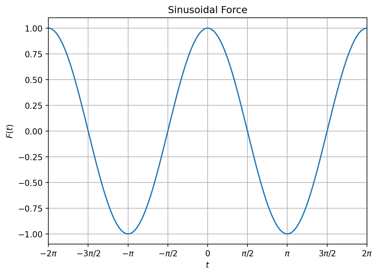
In the previous chapter we looked at a sinusoidal forcing of the type \(F(t) = F_0 cos(\omega t)\). This forcing as seen in Figure 3.1 will repeat itself over time and has a period of \(T = 2\pi/\omega\).
Now let’s consider a funtion \(F(t)\) that is continuous and periodic over the time interval \([-\frac{T}{2}, \frac{T}{2}]\). An example is shown in Figure 3.2, where the function is periodic with a period \(T=2\pi\) but is not sinusoidal.
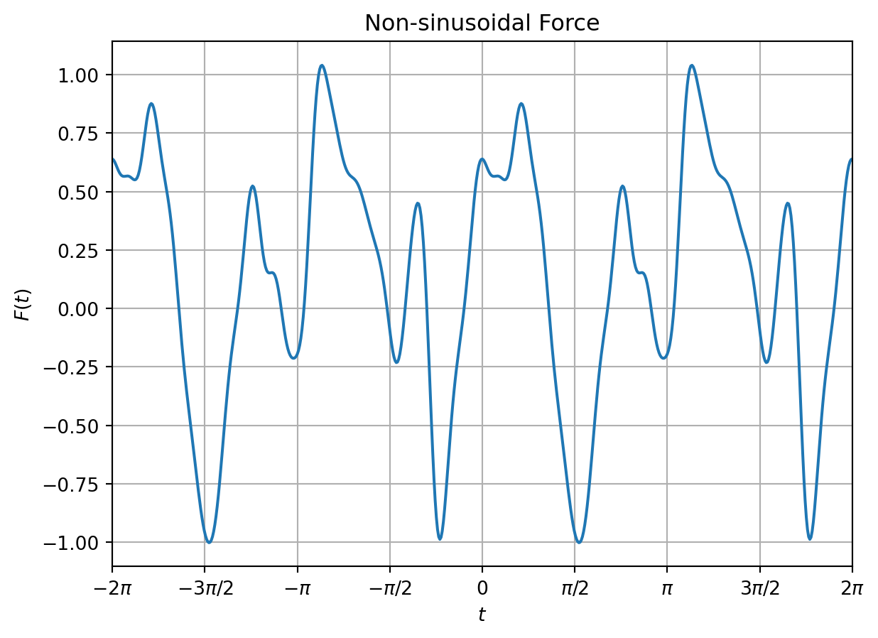
Fourier showed that as long as the function \(F(t)\) is smooth, continuous and periodic, it can be expressed as a trignometric series:
\[\begin{align} F(t) = \frac{a_0}{2} + \sum_{k=1}^{\infty} a_k \cos(k\omega_0 t) + b_k \sin(k\omega_0 t) \label{eq-real-fourier-series} \end{align}\]
where \(\omega_0 = 2\pi/T\) is known as the fundametal frequency of the Fourier series and \(T\) is the fundametal period of the function.
We will now compare this exercise of expressing a function as a Fourier series with the more familiar concept of projecting a vector in 3D vector space along its basis vectors. We know that in 3D space, a vector \(\vec{\boldsymbol{r}}\) is expressed in terms of its projection along the basis vectors as:
\[\begin{align} \vec{\boldsymbol{r}} = a \boldsymbol{\hat{i}} + b \boldsymbol{\hat{j}} + c \boldsymbol{\hat{k}} \end{align}\]
where \(\boldsymbol{\hat{i}}\), \(\boldsymbol{\hat{j}}\) and \(\boldsymbol{\hat{k}}\) are unit vectors along the cardinal directions (\(x\), \(y\) and \(z\) directions) and the values \(a\), \(b\) and \(c\) are the projection of the vector \(\vec{\boldsymbol{r}}\) along \(\boldsymbol{\hat{i}}\), \(\boldsymbol{\hat{j}}\) and \(\boldsymbol{\hat{k}}\).
We can think of a Fourier series as projecting the funtion \(F(t)\) along the basis functions \(\cos(k\omega_0 t)\) and \(\sin(k\omega_0 t)\) for \(k=1,2,...,\infty\). The only difference here is that we are projecting functions into function space and unlike the 3D vector space that has only 3 basis vectors, here we have infinte number of basis functions. The coefficients \(a_k\) and \(b_k\) denote the projection of the function \(F(t)\) along \(\cos(k\omega_0 t)\) and \(\sin(k\omega_0 t)\) respectively.
In the vector space, the cardinal vectors \(\boldsymbol{\hat{i}}\), \(\boldsymbol{\hat{j}}\) and \(\boldsymbol{\hat{k}}\) are orthogonal to each other. This means that when we project one cardinal vector along another, the projection is zero. This idea of projecting one vector along another is denoted by the dot product (or scalar product) operation and the orthogonality is expressed mathematically as:
\[\begin{align} \boldsymbol{\hat{i}}.\boldsymbol{\hat{j}} = \boldsymbol{\hat{i}}.\boldsymbol{\hat{k}} = \boldsymbol{\hat{j}}.\boldsymbol{\hat{k}} = 0 \label{eq-vec-orthogonality} \end{align}\]
The idea of dot product also transfers over to the function spaces. The dot product between two functions \(f(t)\) and \(g(t)\) with domain \([-\frac{T}{2}, \frac{T}{2}]\) is defined as:
\[\begin{align} <f,g> = \int_{-T/2}^{T/2} f(t) g^{*}(t) dt \end{align}\]
where \(g^{*}(t)\) is the complex conjugate of \(g(t)\). If the functions are real valued, then the dot product reduces to:
\[\begin{align} <f,g> = \int_{-T/2}^{T/2} f(t) g(t) dt \end{align}\]
Just as we had the orthogonality of basis vectors as shown in \(\eqref{eq-vec-orthogonality}\), the basis functions \(\cos(k\omega_0 t)\) and \(\sin(k\omega_0 t)\) for \(k=1,2,...,\infty\) are also orthogonal to each other.
\[\begin{align} <\cos(k\omega_0 t), \cos(m\omega_0 t)> &= \int_{-T/2}^{T/2} \cos(k\omega_0 t) \cos(m\omega_0 t) dt \nonumber \\ &= \int_{-T/2}^{T/2} \frac{1}{2}\left\{\cos((k+m)\omega_0 t) + \cos((k-m)\omega_0 t)\right\} dt \nonumber \\ &= \begin{cases} 0 & \text{for } k \neq m \\ \frac{T}{2} & \text{for } k = m \end{cases} \end{align}\]
\[\begin{align} <\sin(k\omega_0 t), \sin(m\omega_0 t)> &= \int_{-T/2}^{T/2} \sin(k\omega_0 t) \sin(m\omega_0 t) dt \nonumber \\ &= \int_{-T/2}^{T/2} \frac{1}{2}\left\{\cos((k-m)\omega_0 t) - \cos((k+m)\omega_0 t)\right\} dt \nonumber \\ &= \begin{cases} 0 & \text{for } k \neq m \\ \frac{T}{2} & \text{for } k = m \end{cases} \end{align}\]
\[\begin{align} <\cos(k\omega_0 t), \sin(m\omega_0 t)> &= \int_{-T/2}^{T/2} \cos(k\omega_0 t) \sin(m\omega_0 t) dt \nonumber \\ &= \int_{-T/2}^{T/2} \frac{1}{2}\left\{\sin((k+m)\omega_0 t) - \sin((k-m)\omega_0 t)\right\} dt \nonumber \\ &= 0 \end{align}\]
Using the orthogonality, the coefficients of the Fourier series can be found as:
\[\begin{align} a_0 &= \frac{2}{T} <F, \cos(0 \times \omega_0 t)> = \frac{2}{T} <F, 1> \\ a_k &= \frac{2}{T} <F, \cos(k \omega_0 t)> \\ b_k &= \frac{2}{T} <F, \sin(k \omega_0 t)> \end{align}\]
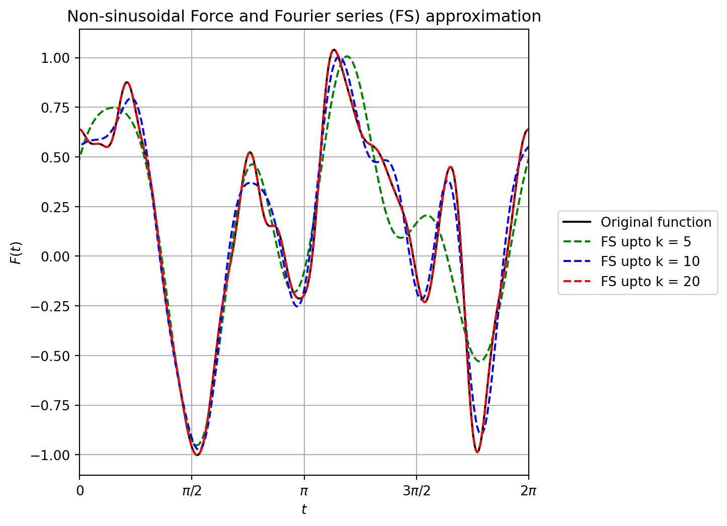
Figure 3.3 shows the Fourier series approximation of the non-sinusoidal function shown in Figure 3.2 as we progressively increase the number of terms considered for summation. It can be seen that with 10 terms the match is fairly good.
3.3 Complex Fourier series
For a real valued function \(F(t)\) defiend over \([-\frac{T}{2}, \frac{T}{2}]\), the Fourier series is given by \(\eqref{eq-real-fourier-series}\). This can further be expressed in terms of complex basis functions as:
\[\begin{align} F(t) &= \frac{a_0}{2} + \sum_{k=1}^{\infty} a_k \cos(k\omega_0 t) + b_k \sin(k\omega_0 t) \nonumber \\ &= \frac{a_0}{2} + \sum_{k=1}^{\infty} \frac{1}{2} \left[(a_k - ib_k)e^{ik\omega_0 t} + (a_k + ib_k)e^{-ik\omega_0 t} \right] \nonumber \\ &= \sum_{k=-\infty}^{\infty} c_k e^{ik\omega_0 t} \end{align}\]
where:
\[\begin{align} c_k = \begin{cases} \frac{1}{2} a_0 & k = 0 \\ \frac{1}{2} (a_k - ib_k) & k > 0 \\ \frac{1}{2} (a_k + ib_k) & k < 0 \end{cases} \end{align}\]
The same principle of orthogonality also holds for the complex basis functions too as shown below:
\[\begin{align} <e^{ik\omega_0 t}, e^{im\omega_0 t}> &= \int_{-T/2}^{T/2} e^{ik\omega_0 t} e^{-im\omega_0 t} dt \nonumber \\ &= \begin{cases} 0 & k \neq m \\ T & k = m \end{cases} \end{align}\]
Using the orthogonality, the coefficients of the Fourier series can be found as:
\[\begin{align} c_k = \frac{1}{T}<F, e^{ik\omega_0 t}> \end{align}\]
It is interesting to note that for a real function \(F(t)\), the complex Fourier coefficients have a symmetry as shown below:
\[\begin{align} c_{-k} = c_k^{*} \end{align}\]
3.4 Fourier transform
The Fourier series we have discussed so far for functions periodic over a finite domain \([-\frac{T}{2}, \frac{T}{2}]\). Note that the consecutive term frequencies are discretely separated by the fundamental frequency \(\omega_0\). The Fourier series can be written as:
\[\begin{align} F(t) &= \sum_{k=-\infty}^{\infty} c_k e^{ik\omega_0 t} \nonumber \\ &= \sum_{k=-\infty}^{\infty} \frac{1}{T}<F, e^{ik\omega_0 t}> e^{ik\omega_0 t} \nonumber \\ &= \sum_{k=-\infty}^{\infty} \frac{\omega_0}{2\pi} \int_{-T/2}^{T/2} F(\xi)e^{-ik\omega_0 \xi} d\xi ~e^{ik\omega_0 t} \end{align}\]
We now extend this idea of Fourier series to functions defined over the domain \((-\infty, \infty)\) by taking the limit \(T \rightarrow \infty\). Note that this means that the fundamental frequency \(\omega_0 \rightarrow d\omega\) and the sum over a discrete set of frequencies (each consecutive one separated by \(\omega_0\)) can be considered as an integral over continuous set of frequencies \(\omega\) in the limit.
\[\begin{align} F(t) &= \lim_{\substack{T\rightarrow \infty \\ \omega_0 \rightarrow d\omega}} \sum_{k=-\infty}^{\infty} \frac{\omega_0}{2\pi} \int_{-T/2}^{T/2} F(\xi)e^{-ik\omega_0 \xi} d\xi ~e^{ik\omega_0 t} \nonumber \\ &= \frac{1}{2\pi} \int_{-\infty}^{\infty} \int_{-\infty}^{\infty} F(\xi)e^{-i\omega \xi} d\xi ~e^{i\omega t} d\omega \end{align}\]
The inner integral is the Fourier transform of the continuous function \(F(t)\) defined over the domain \((-\infty, \infty)\).
\[\begin{align} \hat{F}(\omega) = \mathcal{F}(F(t)) = \int_{-\infty}^{\infty} F(t)e^{-i\omega t} dt \end{align}\]
Similarly the outer integral is the inverse Fourier transform of the continuous function \(\hat{F}(\omega)\) defined over the domain \((-\infty, \infty)\).
\[\begin{align} F(t) = \mathcal{F}^{-1}(\hat{F}(\omega)) = \frac{1}{2\pi} \int_{-\infty}^{\infty} \hat{F}(\omega) e^{i\omega t} d\omega \end{align}\]
The two integrals are known as Fourier transform pair. Both integrals converge as long as \(\int_{-\infty}^{\infty} |F(t)| dt < \infty\) and \(\int_{-\infty}^{\infty} |\hat{F}(\omega)| d\omega < \infty\). The Fourier transform and inverse Fourier transform are both linear operators and accommodate the principle of superposition.
\[\begin{align} \mathcal{F}(af(t) + bg(t)) &= a \mathcal{F}(f) + b \mathcal{F}(g) = a \hat{f}(\omega) + b \hat{f}(\omega) \\ \mathcal{F}^{-1}(a\hat{f}(\omega) + b\hat{g}(\omega)) &= a \mathcal{F}^{-1}(\hat{f}) + b \mathcal{F}^{-1}(\hat{g}) = a f(t) + b f(t) \end{align}\]
The Fourier transform gives us another way to compute the derivative of a function.
\[\begin{align} \frac{dF}{dt} &= \frac{d}{dt} \left(\frac{1}{2\pi}\int_{-\infty}^{\infty} \hat{F}(\omega)e^{i\omega t} d\omega\right) \nonumber\\ &= \frac{1}{2\pi}\int_{-\infty}^{\infty} \hat{F}(\omega)\frac{d}{dt}\left(e^{i\omega t}\right) d\omega \nonumber\\ &= \frac{1}{2\pi}\int_{-\infty}^{\infty} \hat{F}(\omega) i\omega e^{i\omega t} d\omega \nonumber\\ &= \mathcal{F}^{-1}(i\omega \hat{F}(\omega)) \end{align}\]
Thus the Fourier transform of a derivative is equivalent to mulitplying the Fourier transform of the function with \(i\omega\). This usefult property allows converting partial differntial equations into ordinary differential equations. We will use this property later when we discuss hydrodynamics of floating structures.
Another useful property of the Fourier transform is that it converts the convolution operation between two functions in the time domain into a product operation in the frequency domain. The convolution operation between two functions \(f(t)\) and \(g(t)\) is defined as:
\[\begin{align} f * g (t) = \int_{-\infty}^{\infty} f(\tau)g(t - \tau) d\tau \end{align}\]
The Fourier transform of the convolution operation yields:
\[\begin{align} \mathcal{F}(f * g) &= \int_{-\infty}^{\infty} \int_{-\infty}^{\infty} f(\tau)g(t - \tau) d\tau e^{-i\omega t} dt \nonumber \\ &= \int_{-\infty}^{\infty} \int_{-\infty}^{\infty} f(\tau)g(t - \tau) e^{-i\omega (t-\tau)} e^{-i\omega \tau}d\tau dt \nonumber \\ &= \int_{-\infty}^{\infty} \int_{-\infty}^{\infty} f(\tau)g(t - \tau) e^{-i\omega (t-\tau)} dt e^{-i\omega \tau}d\tau \nonumber \\ &= \int_{-\infty}^{\infty} f(\tau) \int_{-\infty}^{\infty} g(\xi) e^{-i\omega \xi} d\xi e^{-i\omega \tau}d\tau \nonumber \\ &= \int_{-\infty}^{\infty} f(\tau) \hat{g}(\omega) e^{-i\omega \tau}d\tau \nonumber \\ &= \int_{-\infty}^{\infty} f(\tau) e^{-i\omega \tau}d\tau \hat{g}(\omega)\nonumber \\ &= \hat{f}(\omega) \hat{g}(\omega) \end{align}\]
Table 3.1 lists some commonly used Fourier transform pairs. Here \(u(t)\) is the unit step function (\(u(t) = 1\) for \(t \geq 0\) and \(0\) otherwise), \(\text{sgn}(t)\) is the signum function (\(\text{sgn}(t) = 1\) for \(t > 0\), \(-1\) for \(t < 0\)) and \(\delta(t)\) is the Dirac delta function.
| Sl. No. | \(f(t)\) | \(\hat{f}(\omega)\) |
|---|---|---|
| 1 | \(\delta(t)\) | \(1\) |
| 2 | \(1\) | \(2\pi\delta(\omega)\) |
| 3 | \(\delta(t - t_0)\) | \(e^{-i\omega t_0}\) |
| 4 | \(e^{i\omega_0 t}\) | \(2\pi\delta(\omega - \omega_0)\) |
| 5 | \(\cos(\omega_0 t)\) | \(\pi\left[\delta(\omega - \omega_0) + \delta(\omega + \omega_0)\right]\) |
| 6 | \(\sin(\omega_0 t)\) | \(\dfrac{\pi}{i}\left[\delta(\omega - \omega_0) - \delta(\omega + \omega_0)\right]\) |
| 7 | \(u(t)\) | \(\pi\delta(\omega) + \dfrac{1}{i\omega}\) |
| 8 | \(\text{sgn}(t)\) | \(\dfrac{2}{i\omega}\) |
| 9 | \(e^{-\alpha t}u(t)\), \(\alpha > 0\) | \(\dfrac{1}{\alpha + i\omega}\) |
| 10 | \(t\,e^{-\alpha t}u(t)\), \(\alpha > 0\) | \(\dfrac{1}{(\alpha + i\omega)^2}\) |
| 11 | \(e^{-\alpha \lvert t \rvert}\), \(\alpha > 0\) | \(\dfrac{2\alpha}{\alpha^2 + \omega^2}\) |
| 12 | \(u(t)\cos(\omega_0 t)\) | \(\dfrac{\pi}{2}\left[\delta(\omega - \omega_0) + \delta(\omega + \omega_0)\right] + \dfrac{i\omega}{\omega_0^2 - \omega^2}\) |
| 13 | \(u(t)\sin(\omega_0 t)\) | \(\dfrac{\pi}{2i}\left[\delta(\omega - \omega_0) - \delta(\omega + \omega_0)\right] + \dfrac{\omega_0}{\omega_0^2 - \omega^2}\) |
| 14 | \(u(t)e^{-\alpha t}\cos(\omega_0 t)\), \(\alpha > 0\) | \(\dfrac{\alpha + i\omega}{(\alpha + i\omega)^2 + \omega_0^2}\) |
| 15 | \(u(t)e^{-\alpha t}\sin(\omega_0 t)\), \(\alpha > 0\) | \(\dfrac{\omega_0}{(\alpha + i\omega)^2 + \omega_0^2}\) |
| 16 | \(f(t) = 1\) for \(\lvert t \rvert < \tau/2\), \(0\) otherwise | \(\dfrac{2\sin(\omega\tau/2)}{\omega}\) |
| 17 | \(f(t) = \dfrac{\sin(Wt)}{\pi t}\) | \(\hat{f}(\omega) = 1\) for \(\lvert \omega \rvert < W\), \(0\) otherwise |
| 18 | \(f(t) = \tau - \lvert t \rvert\) for \(\lvert t \rvert < \tau\), \(0\) otherwise | \(\dfrac{4\sin^2(\omega\tau/2)}{\omega^2}\) |
| 19 | \(e^{-\alpha t^2}\), \(\alpha > 0\) | \(\sqrt{\dfrac{\pi}{\alpha}}\, e^{-\omega^2/4\alpha}\) |
| 20 | \(\displaystyle\sum_{n=-\infty}^{\infty} c_n e^{in\omega_0 t}\) | \(\displaystyle 2\pi\sum_{n=-\infty}^{\infty} c_n \delta(\omega - n\omega_0)\) |
The last entry shows that the Fourier transform of a periodic signal, expressed as a complex Fourier series (as in the previous section), is a train of impulses in the frequency domain located at the harmonics \(n\omega_0\) and weighted by the corresponding Fourier series coefficients \(c_n\).
3.5 Dirac delta function
Consider the first two rows of Table 3.1. It show that the Fourier transform of a constant signal in the time domain is a dirac delta function in the frequency domain and viceversa. This might feel unintuitive at first and needs a closer look to appreciate. Let’s consider a time domain signal that is constant in the range \([-\frac{T}{2},\frac{T}{2}]\) and zero outside. This function is defined mathematically as:
\[\begin{align} f(t) = \begin{cases} 1 & -\frac{T}{2} \leq t \leq \frac{T}{2} \\ 0 & \text{otherwise} \end{cases} \end{align}\]
The Fourier transform of this function is given by:
\[\begin{align} \hat{f}(\omega) &= \int_{-\infty}^{\infty} f(t) e^{-i \omega t} dt \nonumber \\ &= \int_{-T/2}^{T/2} e^{-i \omega t} dt \nonumber \\ &= \frac{e^{-i \omega T/2} - e^{i \omega T/2}}{-i \omega} = T\frac{\sin\left(\frac{\omega T}{2}\right)}{\frac{\omega T}{2}} \nonumber \\ &= T \text{sinc}\left(\frac{\omega T}{2}\right) \label{eq-dirac-fourier} \end{align}\]
Note that the area under the curve is independent of \(T\) as shown below.
\[\begin{align} \int_{-\infty}^{\infty} T \frac{\sin\left(\frac{\omega T}{2}\right)}{\frac{\omega T}{2}} d\omega = 2 \pi \end{align}\]
The animation in Figure 3.4 shows how the Fourier transform \(\hat{f}(\omega)\) shown in \(\eqref{eq-dirac-fourier}\) in the limit \(T \rightarrow 0\) approaches \(2\pi\delta(\omega)\).
3.6 Application to single degree of freedom system
Let’s revisit our differential equation in the forced vibration case:
\[\begin{align} \frac{d^2x}{dt^2} + 2\zeta\omega_n\frac{dx}{dt} + \omega_n^2 x = f(t) = \frac{F(t)}{m} \end{align}\]
Taking a Fourier transform of our differential equation and using the properties of Fourier transform for the derivatives yields:
\[\begin{align} \mathcal{F}(f(t)) &= \mathcal{F} \left(\frac{d^2x}{dt^2} + 2\zeta\omega_n\frac{dx}{dt} + \omega_n^2 x\right) \nonumber \\ \hat{f}(\omega) &= \left((i\omega)^2 + 2\zeta\omega_n (i\omega) + \omega_n^2 \right) \hat{x}(\omega) \nonumber\\ \frac{\hat{x}(\omega)}{\hat{f}(\omega) / \omega_n^2} &= \frac{1}{\left(1 - \frac{\omega^2}{\omega_n^2}\right) + i2\zeta\frac{\omega}{\omega_n}} = H(\omega) \equiv \hat{h} (\omega) \end{align}\]
the same RAO \(\hat{h} (\omega) \equiv H(\omega)\) that we saw in the previous chapter. Thus the Fourier transform of the response \(\hat{x}(\omega)\) is given by:
\[\begin{align} \hat{x}(\omega) = \frac{\hat{h}(\omega) \hat{f}(\omega)}{\omega_n^2} = \frac{\hat{h}(\omega) \hat{F}(\omega)}{k} \end{align}\]
Now we can apply the inverse Fourier transform and use the property of the Fourier transform for the convolution integral to get:
\[\begin{align} x(t) &= \mathcal{F}^{-1}(\hat{x}(\omega)) = \mathcal{F}^{-1}\left(\frac{\hat{h}(\omega) \hat{F}(\omega)}{k}\right) \nonumber \\ &= \frac{1}{k} \int_{-\infty}^{t} F(t) h(t - \tau) d\tau \label{eq-irf-conv} \end{align}\]
where \(h(t) = \mathcal{F}^{-1}(\hat{h}(\omega))\) is known as the impulse response function (IRF) for the system and is the inverse Fourier transform of the RAO. Note the integral upper limit is upto \(t\) and not \(\infty\). This is so to make sure causality is maintained. In physical systems, a force (cause) at a specific time can affect the response (effect) only at that time and in the future. We cannot have a force (cause) in the future affect the response (effect) in the past. Such systems where this cause and effect relationship is maintained are called causal systems. If the upper limit of the integral in \(\eqref{eq-irf-conv}\) is allowed to be \(\infty\), then a force in the future \(F(t')\) with \(t' > t\) can affect the response \(x(t)\) at time \(t\). This breaks causality and is unphysical.
Using the Fourier transform pairs shown in Table 3.1, we can compute the closed form expression for the impulse response function as:
\[\begin{align} h(t) &= \mathcal{F}^{-1}\left(\frac{1}{\left(1 - \frac{\omega^2}{\omega_n^2}\right) + i2\zeta\frac{\omega}{\omega_n}}\right) \nonumber \\ &= \mathcal{F}^{-1}\left(\frac{\omega_n^2}{\left(\omega_n^2 - \omega^2\right) + i2\zeta\omega_n\omega}\right) \nonumber \\ &= \mathcal{F}^{-1}\left(\frac{\omega_n^2}{\left(\zeta\omega_n + i\omega\right)^2 + \omega_n^2(1-\zeta^2)}\right) \nonumber \\ &= \mathcal{F}^{-1}\left(\frac{\omega_n^2}{\omega_n\sqrt{1 - \zeta^2}}\frac{\omega_d}{\left(\zeta\omega_n + i\omega\right)^2 + \omega_d^2}\right) \nonumber \\ &= \frac{\omega_n}{\sqrt{1 - \zeta^2}} e^{-\zeta\omega_nt}\sin(\omega_d t) \end{align}\]
The plot of the impulse response function for \(\omega_n = 3.0\) rad/s and \(\zeta=0.1\) is shown in Figure 3.5.
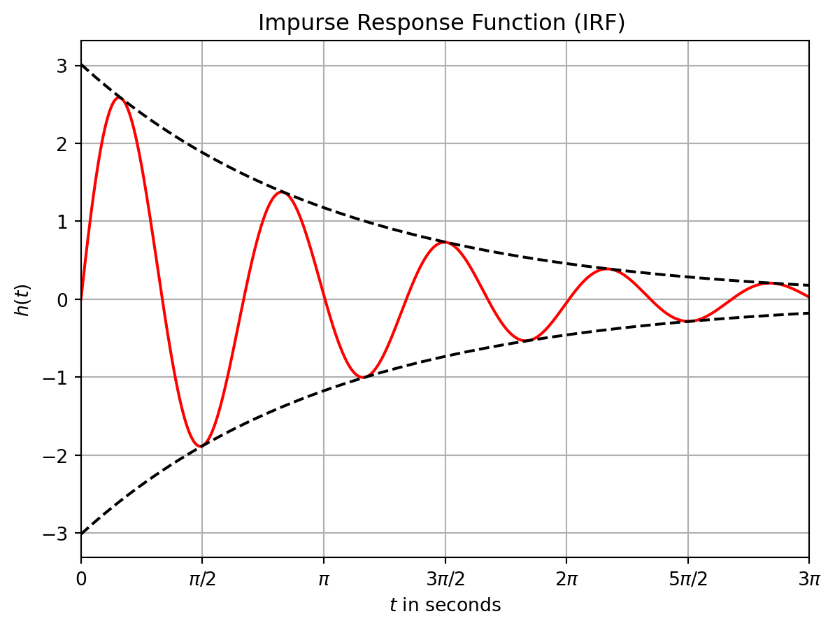
Note that this response shown in Figure 3.5 is the response of the mass when the input excitation is \(F(t) = k\delta(t)\) where \(\delta(t)\) is the Dirac delta function or the impulse function. The Dirac delta is zero everywhere except where the argument of the function is zero (in this case \(t=0\)).
Notion of sum of impluses
A general force time history can be thought of as an infinite series of impulses of strength \(F(\tau)\) at each time \(\tau\). The total response \(x(t)\) at some time \(t\) is then the sum of the individual responses to each of these impulses summed at time \(t\) due to all the impulses that came prior to time \(t\). Response of one impulse that occured at time \(\tau\) is \(F(\tau)h(t-\tau)/k\) and affects the total response for all \(t>\tau\). We need to sum across all impulses that happended at all times \(\tau < t\). This is given by the following (which turns out to be the convolution integral):
\[\begin{align} x(t) = \frac{1}{k} \int_{-\infty}^{t} F(\tau)h(t-\tau) d\tau \label{eq-convolution-irf} \end{align}\]
The animation in Figure 3.6 illustrates this superposition: each impulse at time \(\tau\) contributes a response \(F(\tau)h(t-\tau)/k\) for \(t > \tau\), and the total \(x(t)\) is the sum of all such contributions.
Notice that this a huge improvement as compared to our previous chapter. There we were restricted to only sinusoidal forcing. But now for any irregular forcing \(F(t)\) we can compute the response \(x(t)\) of our single degree of freedom system.
In general computing the convolution term shown in \(\eqref{eq-convolution-irf}\) is computationally expensive as we need to slide one signal across the other and for each sliding offset we multiply the functions and calculate the area under it. The same process in Fourier domain is a lot cheaper as it is simply a multiplication of the Fourier transfrom of the functions. In adopting the computation in the Fourier domain we are essentially separating the irregular force time history into its component regular waves (through Fourier transform), computing the response of each of these regular wave components and summing them together (inverse Fourier transform) to get the response to the irregular force.
3.7 Exercises
Unless stated otherwise use \(\rho = 1025\) kg/m\(^3\) and \(g = 9.81\) m/s\(^2\). Every problem below can be solved with the Fourier series and Fourier transform results of this chapter, the single degree of freedom results of Chapter 2 (free vibration, the RAO \(H(\omega)\), the principle of superposition) and the elementary hydrostatics you already know. Wherever a hydrodynamic force acts, its amplitude is given to you: added mass, radiation damping and wave loading are not required. The two results from linear wave theory that are quoted in Problem 4 — the deep water wavelength \(\lambda = gT^2/2\pi\) and the crest speed \(c = gT/2\pi\) — are stated there for you to use and will be derived in a later chapter.
Several problems ask you to derive a result before using it numerically; the derivation carries most of the marks. The principal dimensions are representative rather than exact and are used only to give the numbers a realistic scale.
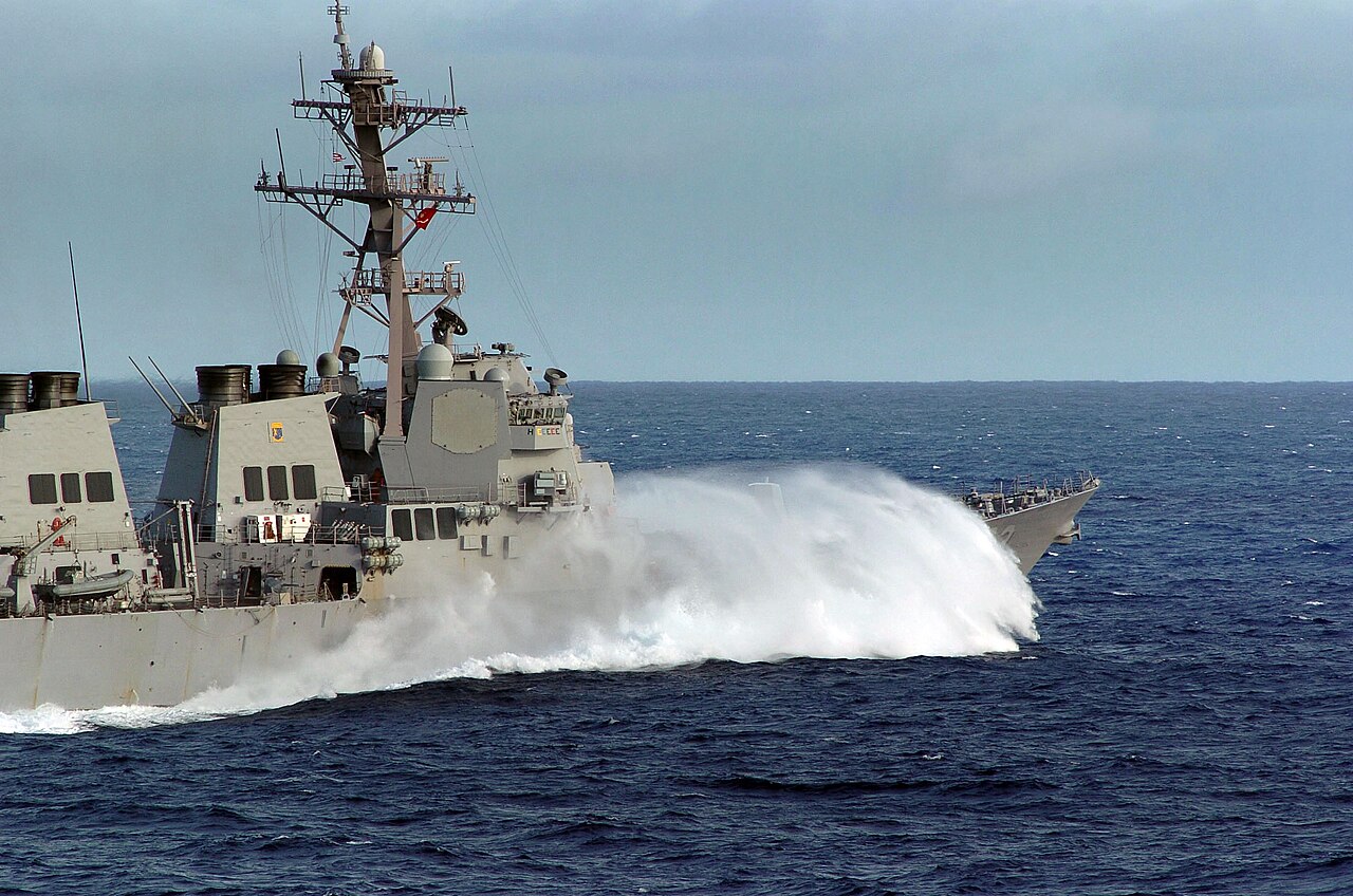
Two of the problems below concern forces that arrive as a repeating series of short blows rather than as a smooth wave. Figure 3.7 shows the physical situation. A ship driving into head seas buries her bow in a wave every few seconds; the flare of the bow strikes the water surface, and the resulting impulse is severe, brief and repeated once per wave encounter. This is the loading idealised in Problem 2, and the whole point of that problem is that a force made of short pulses carries energy at frequencies far above the wave frequency that produced it.
A thruster that cannot make up its mind. A moored construction barge is held on station in surge by a thruster that is controlled in an on–off (bang–bang) manner: it delivers a constant thrust \(F_0 = 900\) kN for exactly half of every cycle and nothing for the other half, the cycle period being \(T = 60\) s. The barge has an effective surge mass \(m = 2.4\times10^{7}\) kg, a surge natural period of \(20\) s and \(\zeta = 0.05\).
- Using the orthogonality relations of this chapter, derive the Fourier series of this on–off thrust. Show that \(a_0/2 = F_0/2\), that \(a_k = 0\) for all \(k \geq 1\), and that \(b_k = 2F_0/(k\pi)\) for odd \(k\) and zero for even \(k\). Explain, from the symmetry of \(F(t) - F_0/2\) about the time axis, why the even harmonics must be absent.
- Compute the mooring stiffness and the mean surge offset. For each of the harmonics \(k = 1, 3, 5, 7\) compute \(\omega_k\), the force amplitude, the frequency ratio \(r_k\), \(|H(\omega_k)|\), the phase and the response amplitude. Present the results as a table.
- Which harmonic dominates the motion, and why? Sum the series numerically to obtain the largest and smallest surge excursion in a cycle, and compare with the naive estimate “mean thrust divided by stiffness”.
- The operator proposes two fixes, both of which keep the mean thrust at \(450\) kN so that station-keeping is unaffected: (i) reduce the on-fraction to \(d = 1/3\) and raise the thrust to \(1350\) kN; (ii) keep \(d = 1/2\) and \(F_0 = 900\) kN but shorten the cycle period to \(45\) s. First show that for a general on-fraction \(d\) the \(k\)-th harmonic has amplitude \(2F_0\lvert\sin(\pi k d)\rvert/(\pi k)\), so that the \(k\)-th harmonic vanishes whenever \(kd\) is an integer. Then evaluate both proposals and recommend one.
- State the general lesson about eliminating a single offending harmonic.
A ship’s hull is not rigid: it rings like a beam. The lowest elastic mode of a hull girder is the two-node vertical mode sketched in Figure 3.8, in which the bow and stern move one way while amidships moves the other, and two stations along the length stay still. A slam at the bow excites this mode, and the resulting vibration — whipping — is what Problem 2 analyses. Its natural frequency is far above the wave frequencies of Figure 3.7, which is exactly why the harmonic content of a short pulse matters.
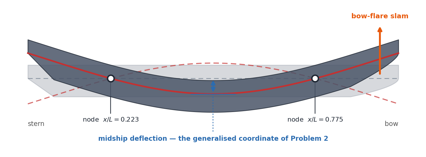
Bow slamming and the whipping of a hull girder. A ship steaming in head seas takes a bow-flare slam once every wave encounter, the encounter period being \(T_e = 7.5\) s. Each slam is idealised as a rectangular force pulse of magnitude \(F_0 = 15\) MN and duration \(\tau = 0.20\) s, repeating with period \(T_e\). The two-node vertical vibration mode of the hull girder behaves as a single degree of freedom system with generalised mass \(M = 1.2\times10^{7}\) kg, natural frequency \(1.10\) Hz and \(\zeta = 0.012\); the generalised coordinate may be read as the midship vertical deflection.
- Show that the \(k\)-th harmonic of a rectangular pulse train with on-fraction \(d = \tau/T_e\) has amplitude \(2F_0\lvert\sin(\pi k d)\rvert/(\pi k)\), and hence that for \(d \ll 1\) this is very nearly \(2F_0\tau/T_e\) — the same for every harmonic — until the envelope first vanishes at \(\omega = 2\pi/\tau\). Compute that frequency and the number of harmonics lying below it. Explain in one sentence why “a short blow is broadband”.
- Compute the modal stiffness, \(\omega_0\) and \(\omega_n/\omega_0\). Tabulate the force amplitude, \(r_k\), \(|H_k|\) and the modal response for \(k = 1, 2, 8, 9, 10\). Compare the wave-frequency (\(k=1\)) deflection with the \(k=8\) deflection and comment.
- Sum the series numerically and report the largest and smallest midship deflection, and the sum \(\sum_k |x_k|\). Why is the sum a poor estimate of the peak?
- In heavier weather the slam duration doubles to \(\tau = 0.4\) s at the same peak force. Recompute the \(k=8\) response. Then find the slam duration that would place a zero of the envelope exactly on the eighth harmonic. Is such a duration physically achievable for a slam? What does this tell you about trying to “detune” a slam?
- The master reduces speed, changing the encounter period. Compute the largest single-harmonic response for \(T_e = 6.0, 7.0, 7.5, 8.0\) and \(9.0\) s, and find the two encounter periods near \(7.5\) s that place a harmonic exactly on \(\omega_n\). What is the worst case, and what is the only reliable remedy?
How many harmonics do you actually need? Every practical calculation truncates the Fourier series. This problem establishes how to decide where to stop.
- Starting from the orthogonality relations, show that for a real periodic \(F(t)\) \[\overline{F^2} \equiv \frac{1}{T}\int_{-T/2}^{T/2} F^2(t)\,dt = \frac{a_0^2}{4} + \frac{1}{2}\sum_{k=1}^{\infty}\left(a_k^2 + b_k^2\right) = \sum_{k=-\infty}^{\infty}\lvert c_k\rvert^2\] This is Parseval’s theorem: the mean square of a signal is the sum of the mean squares of its harmonics, and no cross terms survive.
- Apply it to a zero-mean square wave of amplitude \(\pm F_0\), for which \(b_k = 4F_0/(k\pi)\) for odd \(k\). Verify that the series sums exactly to \(F_0^2\), then compute the fraction of the mean square captured by harmonics up to \(k = 1, 3, 5, 7\) and find how many non-zero terms are needed for \(99\%\) and for \(99.9\%\).
- Repeat for a triangular wave of the same peak value, for which \(a_k = 8F_0/(\pi^2k^2)\) for odd \(k\) and \(\overline{F^2} = F_0^2/3\). Explain the very different convergence rate in terms of the smoothness of the two waveforms, and say which is the better model of a real wave force.
- Now apply Parseval to the response of the barge of Problem 1. Compute the share of the mean-square surge carried by each harmonic and the number of harmonics needed for \(99\%\) of it. Compare with your answer to (b).
- Repeat (d) for a stiff bottom-founded structure excited by the same square-wave force but with \(\omega_n = 15\,\omega_0\). State the practical rule for choosing the number of harmonics to retain.
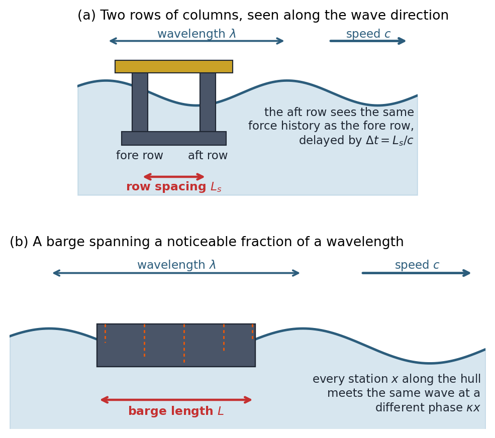
Problem 4 turns on a single idea: the same wave reaches different parts of a structure at different times, and a delay in time is a phase shift in frequency. Figure 3.9 shows the two arrangements the problem treats. Read it before starting, because the geometry is the whole difficulty — the algebra afterwards is just the shift property.
Column spacing, barge length and the cancellation period. Two consequences of the shift property, both of them used in real hull-form design. Throughout, use the deep-water results \(\lambda = gT^2/2\pi\) for the wavelength, \(c = gT/2\pi\) for the crest speed and \(\kappa = 2\pi/\lambda = \omega^2/g\) for the wavenumber; these will be derived in a later chapter.
- Prove the shift property \(\mathcal{F}\left(f(t-t_0)\right) = e^{-i\omega t_0}\hat{f}(\omega)\) directly from the definition, and note that \(\left\lvert e^{-i\omega t_0}\right\rvert = 1\): a pure delay changes only phase.
- A semi-submersible has two rows of columns, a distance \(L_s = 60\) m apart along the wave direction. Each row carries the same vertical wave force history, the aft row delayed by the time the crest takes to travel between them, \(\Delta t = L_s/c\). Show that the total force satisfies \(\hat{F}_{tot}(\omega) = \hat{F}(\omega)\left(1 + e^{-i\omega\Delta t}\right)\) with \(\left\lvert 1 + e^{-i\omega\Delta t}\right\rvert = 2\left\lvert\cos(\kappa L_s/2)\right\rvert\), and hence that the total force vanishes when \(L_s = \lambda/2\). Tabulate the gain for wave periods \(6, 8, 10, 12, 14\) and \(16\) s and find the cancellation period.
- The site has a peak wave period of \(10\) s. What row spacing places the cancellation there? Comment on why a designer cannot simply choose the spacing on this basis alone.
- In reality the aft row is partly shielded and receives only \(0.85\) of the force of the fore row. Recompute the gain at the cancellation period. How good is the cancellation now?
- A rectangular barge of length \(L = 100\) m, beam \(B = 24\) m and draft \(5\) m floats freely in head seas. The vertical wave force per unit length is \(f(x,t) = f_0\cos(\kappa x - \omega t)\) with \(f_0 = 55\) kN/m, taken independent of frequency for this exercise, and \(x\) measured from midships. Show that the total heave force is \(F(t) = f_0 L\,\mathrm{sinc}(\kappa L/2)\cos(\omega t)\), and identify this result with entry 16 of Table 3.1 with \((t,\omega)\) replaced by \((x,\kappa)\). Compute the barge’s heave natural period and \(\zeta = 0.20\) response amplitude at wave periods from \(5.66\) s to \(16\) s, and explain the two zeros you find.
Reading a decay test in the frequency domain. A spar platform is displaced in heave and released, and the decay is recorded. The measured record is well fitted by \(x(t) = X_0e^{-\zeta\omega_nt}\cos(\omega_dt)\) for \(t \geq 0\) with \(X_0 = 1.80\) m. The first positive peak is \(1.80\) m, the sixth is \(0.60\) m, and the two are \(140.1\) s apart. The amplitude spectrum \(\lvert\hat{x}(\omega)\rvert\) computed from the same record peaks at \(\omega = 0.2243\) rad/s and falls to \(1/\sqrt{2}\) of its peak value at \(\omega = 0.2164\) and \(0.2321\) rad/s.
- Using entry 14 of Table 3.1, write \(\hat{x}(\omega)\). Show that near the peak \(\lvert\hat{x}(\omega)\rvert \approx \dfrac{X_0/2}{\sqrt{(\omega_d-\omega)^2 + (\zeta\omega_n)^2}}\), and hence that the two half-power points are separated by \(\Delta\omega = 2\zeta\omega_n\). This is the half-power bandwidth method of extracting damping.
- Determine \(\zeta\), \(\omega_n\) and \(T_n\) from the spectrum. Independently determine \(\zeta\), \(T_d\) and \(\omega_n\) from the time-domain peaks by logarithmic decrement, and compare.
- The record was sampled for \(600\) s. Compute the time for the decay envelope to fall to \(1\%\) of its initial value, the frequency spacing \(\Delta\omega = 2\pi/T_{rec}\) of the Fourier coefficients of a \(600\) s record, and the number of spectral points that fall inside the half-power band. How long a record would you need for five points across the band, and is simply recording for longer the right answer? Justify your reasoning physically.
- The same record also contains the mooring-controlled surge mode, which appears as \(0.50\,e^{-\zeta_2\omega_2t}\cos(\omega_2t)\) with \(\omega_2 = 0.090\) rad/s and \(\zeta_2 = 0.10\). Compute the contribution of this second mode to \(\lvert\hat{x}\rvert\) at the heave peak frequency, as a percentage. Why is the frequency-domain estimate of damping more robust than the logarithmic decrement for a record containing two modes?
- Show that the product of the decay time to \(1\%\) and the half-power bandwidth is \(2\ln 100 = 9.21\), independent of \(\zeta\) and \(\omega_n\). Evaluate both quantities for this spar, for the same spar fitted with heave plates (\(\zeta = 0.15\)) and for a jacket sway mode (\(T_n = 4\) s, \(\zeta = 0.03\)), and state the principle in words.
A squall on a moored FPSO. A moored FPSO has an effective surge mass of \(2.8\times10^{8}\) kg, a total mooring stiffness of \(1.2\times10^{6}\) N/m and \(\zeta = 0.08\). It is initially at rest at its equilibrium position when a squall raises the wind force from zero to \(F_0 = 3.0\) MN, effectively instantaneously. The most heavily loaded mooring line carries a pretension of \(2.0\) MN and its tension rises by \(0.75\) MN for every metre of surge offset; the maximum allowable tension is \(5.0\) MN.
- Using the convolution integral \(\eqref{eq-convolution-irf}\) with the impulse response function derived in this chapter, show that the response to a step force applied at \(t=0\) is \[x(t) = \frac{F_0}{k}\left[1 - e^{-\zeta\omega_nt}\left(\cos\omega_dt + \frac{\zeta\omega_n}{\omega_d}\sin\omega_dt\right)\right]\]
- Compute \(\omega_n\), \(T_n\) and the static offset. Show that the maximum occurs at \(t = \pi/\omega_d\) with a dynamic amplification factor \(\mathrm{DAF} = 1 + e^{-\pi\zeta/\sqrt{1-\zeta^2}}\), evaluate it, and check the mooring line tension against its allowable value both statically and dynamically.
- The squall in fact lasts a finite time \(t_d\) before the wind drops again. Explain how superposition gives the response as the difference of two step responses, and compute the DAF for \(t_d/T_n = 0.1, 0.25, 0.5, 1.0\) and \(2.0\). Compare with the undamped result \(\mathrm{DAF} = 2\sin(\pi t_d/T_n)\) for \(t_d < T_n/2\), and explain why the DAF stops growing once \(t_d\) exceeds \(T_n/2\).
- Squalls at the site last several minutes. Which of your cases applies, and what is the worst credible offset?
- A real squall does not rise instantaneously. Take instead a force that ramps linearly from \(0\) to \(F_0\) over a time \(t_r\) and then stays constant, and compute the peak offset for \(t_r/T_n = 0.25, 0.5, 1.0\) and \(2.0\) by evaluating the convolution numerically. What property of the loading, rather than its magnitude, decides whether a structure responds dynamically?
Displacement, velocity and acceleration are three different spectra. The measured vertical motion of the bridge deck of a ship is analysed over a record and found to consist of the following harmonic components. The first four are wave-frequency motions; the fifth is the hull-girder whipping component of Problem 2.
component 1 2 3 4 5 \(\omega_j\) (rad/s) 0.35 0.52 0.70 0.95 6.912 \(X_j\) (m) 1.20 0.60 0.30 0.18 0.020 Crane operations must be suspended if the RMS vertical acceleration exceeds \(0.05g\).
- Using the derivative property of the Fourier transform, show that if \(x\) has a component of amplitude \(X_j\) at frequency \(\omega_j\) then \(\dot{x}\) and \(\ddot{x}\) have components of amplitude \(\omega_jX_j\) and \(\omega_j^2X_j\) at the same frequency, and state the corresponding relation between the complex Fourier coefficients \(c_k\) of a periodic signal and those of its derivatives.
- Tabulate the displacement, velocity and acceleration amplitude of each component. Which component is largest in each of the three quantities?
- Using Parseval’s theorem from Problem 3, compute the RMS displacement, velocity and acceleration. Must crane operations be suspended?
- Compute the share of the displacement variance and of the acceleration variance carried by the whipping component. Comment on the size of the two numbers.
- By what factor must the whipping amplitude be reduced for the criterion to be met? Compare with the effect of halving the largest wave-frequency component instead. What does this imply about a motion sensor, or a numerical model, that resolves only the wave frequency band?
The memory of the convolution. The convolution \(\eqref{eq-convolution-irf}\) says that the response now depends on the entire past of the force. This problem asks how much of that past actually matters, and what it costs.
- Verify from \(h(t) = \dfrac{\omega_n}{\sqrt{1-\zeta^2}}e^{-\zeta\omega_nt}\sin(\omega_dt)\) that \(h(0) = 0\), \(\dot{h}(0) = \omega_n^2\) and \(\displaystyle\int_0^{\infty}h(t)\,dt = 1\). Interpret the last result physically by comparing it with \(H(0)\).
- Define the memory time \(t_m\) as the time for the envelope of \(h\) to fall to \(1\%\) of its initial value. Show that \(t_m = \ln(100)/(\zeta\omega_n)\) and that the corresponding number of cycles is \(\ln(100)/(2\pi\zeta)\), independent of \(\omega_n\). Evaluate \(t_m\) in seconds and in cycles for: FPSO surge (\(T_n = 96\) s, \(\zeta = 0.08\)); bare spar heave (\(T_n = 28\) s, \(\zeta = 0.035\)); the same spar with heave plates (\(\zeta = 0.15\)); jacket sway (\(T_n = 4\) s, \(\zeta = 0.03\)).
- A three-hour simulation is run with a time step of \(0.1\) s. For each of the four modes, estimate the number of multiply–add operations needed to evaluate the convolution at every time step over the memory time, and compare with the \(5N\log_2N\) operations of an FFT-based frequency-domain solution of the whole record.
- Show that truncating the memory at \(t_m\) leaves an error bounded by \(\dfrac{F_{max}}{k}\dfrac{e^{-\zeta\omega_nt_m}}{\zeta\sqrt{1-\zeta^2}}\). For the bare spar with \(F_{max}/k = 0.5\) m, find the memory time needed to guarantee an error below \(1\) mm and compare it with the \(1\%\) envelope rule of part (b). Which is the safer criterion, and why do the two differ so much?
- Which mode is the most expensive to simulate in the time domain, and why is it also the one for which the frequency-domain approach is most attractive? Relate your answer to the number of cycles needed to build up a resonant response.
Two swells that are nearly the same. A moored structure is excited in heave by two swell systems arriving from nearly the same direction, giving a heave force \[F(t) = F_1\cos(\omega_1t) + F_2\cos(\omega_2t), \qquad F_1 = F_2 = 0.60~\text{MN}\] with \(\omega_1 = 0.480\) rad/s and \(\omega_2 = 0.520\) rad/s. The structure has an effective heave mass of \(4.2\times10^{7}\) kg, \(\omega_n = 0.50\) rad/s and \(\zeta = 0.02\).
- Show that \(F(t) = 2F_1\cos\left(\frac{\Delta\omega}{2}t\right)\cos\left(\bar{\omega}t\right)\) with \(\bar{\omega} = (\omega_1+\omega_2)/2\) and \(\Delta\omega = \omega_2-\omega_1\), and write down \(\hat{F}(\omega)\) using Table 3.1. Compute the group period, the carrier period and the number of waves per group.
- Compute the heave stiffness, and the amplitude and phase of each response component.
- Show that the response is also a beat, and compute the maximum and minimum of its envelope and the modulation depth \((\max-\min)/(\max+\min)\). Why is the minimum not zero, when the force envelope falls exactly to zero?
- Show that the response envelope peaks a time \(-\Delta\phi/\Delta\omega\) after the force envelope, where \(\Delta\phi = \phi_2-\phi_1\), and evaluate it. Verify numerically. Explain why the largest response does not occur when the largest wave group arrives.
- Recompute the number of waves per group for frequency separations \(\Delta\omega = 0.08, 0.04\) and \(0.02\) rad/s, and use the build-up result \(N_{95} = \ln(20)/(2\pi\zeta)\) from the previous chapter to find what fraction of the steady-state amplitude each group actually delivers. Which sea is the dangerous one, and what does this say about the steady-state answers computed in (b) and (c)?
Programming Problem: Three routes to the same answer. A slender compliant offshore tower has an effective mass of \(6.0\times10^{6}\) kg, a natural frequency \(\omega_n = 1.80\) rad/s and \(\zeta = 0.04\). In an oscillatory flow the horizontal force on a slender member is proportional to \(u\lvert u\rvert\), where \(u\) is the flow velocity — a result you will meet later, and which you should simply take as given here. With a wave of frequency \(\omega_0 = 0.60\) rad/s the horizontal force on the tower is therefore \[F(t) = F_0\cos(\omega_0t)\left\lvert\cos(\omega_0t)\right\rvert, \qquad F_0 = 1.2~\text{MN}\]
- Explain from the symmetries of \(F(t)\) why its Fourier series contains only odd cosine harmonics. Compute \(a_1, a_3, a_5, a_7\) numerically, by direct quadrature of the Fourier integrals and again with
numpy.fft.rfftapplied to one period, and compare \(a_1\) with the classical value \(8/(3\pi)\). Confirm that the even harmonics are zero to machine precision. - Compute the tower stiffness and \(\omega_n/\omega_0\). Tabulate the force amplitude, \(r_k\), \(\lvert H_k\rvert\) and the response amplitude of each harmonic up to \(k=6\), and report \(\sum_k\lvert x_k\rvert\) and \(\max\lvert x(t)\rvert\) obtained by summing the series.
- Solve the same problem in the time domain by evaluating the convolution \(\eqref{eq-convolution-irf}\) numerically with the impulse response function (
numpy.convolveis the natural tool). Run for \(140\) s, discard the first \(90\) s as transient and compare the steady-state maximum with (b). Repeat with \(\Delta t = 0.2, 0.1, 0.05, 0.02\) and \(0.01\) s and comment on the convergence. - Solve it a third time by integrating the equation of motion directly with a fourth-order Runge–Kutta scheme, and report the largest difference between the three solutions in the steady state.
- A common engineering shortcut replaces the drag force by an equivalent linear force retaining only the fundamental harmonic. What response does that shortcut predict, and by what factor is it in error? Explain precisely which piece of physics it discards.
- The ship moves to a site where the same tower sees waves of \(\omega_0 = 0.90\) rad/s, so that \(\omega_n = 2\omega_0\) exactly, the force amplitude being unchanged. Predict, before computing, whether the response will be larger or smaller, then compute \(\sum_k\lvert x_k\rvert\) and explain the result.
- Finally, repeat the FFT of part (a) over a window of \(4.0\) periods and then of \(4.3\) periods, and plot or list the resulting amplitude at each bin. Explain what you see in terms of the assumption that underlies every Fourier series.
- Explain from the symmetries of \(F(t)\) why its Fourier series contains only odd cosine harmonics. Compute \(a_1, a_3, a_5, a_7\) numerically, by direct quadrature of the Fourier integrals and again with
Answer Key
Problem 1 — A thruster that cannot make up its mind
(a) \(a_0 = \frac{2}{T}\int_0^{T/2}F_0\,dt = F_0\), so the mean thrust is \(a_0/2 = F_0/2\). For \(k\geq1\), \(a_k = \frac{2F_0}{T}\int_0^{T/2}\cos(k\omega_0t)dt = \frac{2F_0}{k\omega_0T}\sin(k\pi) = 0\) and \(b_k = \frac{2F_0}{T}\int_0^{T/2}\sin(k\omega_0t)dt = \frac{F_0}{k\pi}\left[1-(-1)^k\right]\), which is \(2F_0/(k\pi)\) for odd \(k\) and \(0\) for even \(k\). The reason is a symmetry: \(F(t)-F_0/2\) satisfies \(F(t+T/2)-F_0/2 = -\left[F(t)-F_0/2\right]\) (half-wave antisymmetry). Every even harmonic \(\cos(2j\omega_0t)\), \(\sin(2j\omega_0t)\) repeats itself after \(T/2\) and is therefore orthogonal to any half-wave antisymmetric function, so its coefficient must vanish. A square wave contains only odd harmonics.
(b) \(\omega_n = 2\pi/20 = 0.31416\) rad/s, \(k = m\omega_n^2 = 2.3687 \times 10^{6}\) N/m, \(\omega_0 = 2\pi/60 = 0.10472\) rad/s and note \(\omega_n = 3\omega_0\) exactly. Mean offset \(= (F_0/2)/k = 0.1900\) m.
| \(k\) | \(\omega_k\) (rad/s) | \(F_k\) (kN) | \(r_k\) | \(\lvert H_k\rvert\) | \(\phi_k\) (deg) | \(\lvert x_k\rvert\) (m) |
|---|---|---|---|---|---|---|
| 1 | 0.1047 | 573.0 | 0.3333 | 1.1242 | -2.1 | 0.2719 |
| 3 | 0.3142 | 191.0 | 1.0000 | 10.0000 | -90.0 | 0.8063 |
| 5 | 0.5236 | 114.6 | 1.6667 | 0.5600 | -174.6 | 0.0271 |
| 7 | 0.7330 | 81.9 | 2.3333 | 0.2247 | -177.0 | 0.0078 |
(c) The third harmonic dominates: it carries only \(191\) kN, one third of the fundamental, but it sits exactly on resonance (\(r_3 = 1\), \(|H_3| = 1/2\zeta = 10\)) and produces \(0.806\) m against the fundamental’s \(0.272\) m. Summing the series, the surge ranges from \(-0.863\) m to \(1.243\) m, a peak-to-peak excursion of \(2.106\) m about a mean offset of only \(0.190\) m. A quasi-static estimate based on the mean thrust alone understates the largest offset by a factor of \(6.5\). The thruster never excites the barge at \(\omega_n\), yet the barge responds almost entirely at \(\omega_n\).
(d) Over one period the thrust is \(F_0\) for \(0<t<dT\) and zero afterwards, so \(c_k = \frac{F_0}{T}\int_0^{dT}e^{-ik\omega_0t}dt = \frac{F_0\left(1-e^{-i2\pi kd}\right)}{i2\pi k}\) and the amplitude of the \(k\)-th real harmonic is \(2|c_k| = \dfrac{2F_0\lvert\sin(\pi kd)\rvert}{\pi k}\), which vanishes whenever \(kd\) is an integer. Setting \(d = 1/2\) recovers part (a).
Proposal (i) (\(d = 1/3\), \(F_0 = 1350\) kN): the third harmonic is now exactly zero, but even harmonics appear where there were none. \(|x_1| = 0.3532\) m, \(|x_2| = 0.2808\) m, \(|x_3| = 0\), \(|x_4| = 0.0995\) m, giving \(\sum_k|x_k| = 0.7931\) m against \(1.1131\) m originally — an improvement of only \(29\%\). Two things spoil it: the amplitude had to be raised by \(50\%\) to hold the mean thrust, and the second harmonic at \(r_2 = 2/3\) is still strongly amplified (\(|H| = 1.79\)).
Proposal (ii) (\(T = 45\) s): now \(\omega_0 = 0.13963\) rad/s and the odd harmonics sit at \(r = 0.444, 1.333, 2.222,\ldots\) — none of them near resonance. \(|x_1| = 0.3010\) m, \(|x_3| = 0.1022\) m, \(|x_5| = 0.0123\) m and \(\sum_k|x_k| = 0.4240\) m, a reduction by a factor of \(2.6\). Recommend (ii).
(e) Killing one harmonic is not the same as killing the response. The Fourier coefficients of a periodic signal are constrained by its shape and its mean; forcing one of them to zero while holding the mean fixed pushes energy into its neighbours, and the neighbours may be amplified almost as strongly. The robust fix is to move the whole comb of harmonics \(k\omega_0\) so that no member of it lands near \(\omega_n\) — that is, to change the repetition period rather than the pulse shape.
Problem 2 — Bow slamming and the whipping of a hull girder
(a) From Problem 1(d), \(2|c_k| = 2F_0|\sin(\pi kd)|/(\pi k)\). Writing \(\pi k d = \pi k\tau/T_e\) and using \(\sin u \approx u\) for \(u \ll 1\) gives \(2|c_k| \approx 2F_0\tau/T_e = 0.8000\) MN, independent of \(k\): the pulse train has a flat spectrum whose height is set by the impulse \(F_0\tau = 3.0\) MN·s and not by the peak force alone. The envelope first vanishes when \(\pi k d = \pi\), i.e. at \(\omega = k\omega_0 = 2\pi/\tau = 31.42\) rad/s (\(f = 5.0\) Hz), which is harmonic \(k = T_e/\tau = 37.5\). So roughly \(9\) harmonics lie within \(10\%\) of the flat value. The shorter the blow, the wider the band of frequencies it excites — and a \(0.2\) s blow reaches frequencies an order of magnitude above the wave frequency, where the hull girder lives.
(b) \(\omega_n = 2\pi(1.10) = 6.9115\) rad/s, \(k_m = M\omega_n^2 = 5.7323 \times 10^{8}\) N/m, \(\omega_0 = 0.8378\) rad/s, \(\omega_n/\omega_0 = 8.250\) — so harmonics \(8\) and \(9\) straddle the natural frequency. Mean force of the train \(= F_0d = 0.40\) MN, giving a static offset of only \(0.70\) mm.
| \(k\) | \(\omega_k\) (rad/s) | \(F_k\) (MN) | \(r_k\) | \(\lvert H_k\rvert\) | \(\lvert x_k\rvert\) (mm) |
|---|---|---|---|---|---|
| 1 | 0.8378 | 0.7991 | 0.1212 | 1.015 | 1.41 |
| 2 | 1.6755 | 0.7963 | 0.2424 | 1.062 | 1.48 |
| 8 | 6.7021 | 0.7414 | 0.9697 | 15.609 | 20.19 |
| 9 | 7.5398 | 0.7263 | 1.0909 | 5.212 | 6.60 |
| 10 | 8.3776 | 0.7097 | 1.2121 | 2.127 | 2.63 |
The wave-frequency component deflects the hull by \(1.41\) mm; the eighth harmonic, which carries a force of the same size, deflects it by \(20.19\) mm — \(14\) times more, purely because \(|H|\) is \(15.6\) there instead of \(1.01\). This is whipping: a high-frequency ringing of the hull girder at about \(1\) Hz superimposed on the slow wave-frequency bending. - (c) \(\sum_k|x_k| = 52.0\) mm, but the actual record runs from \(-24.9\) mm to \(33.0\) mm, i.e. only \(63\%\) of the bound. The bound is loose because the harmonics that dominate the sum are near resonance and are phase-shifted by roughly \(-90^\circ\) relative to the rest, so the components never all peak together. - (d) With \(\tau = 0.4\) s the eighth harmonic grows to \(1.1621\) MN and the response to \(31.6\) mm — a factor \(1.57\) worse, because the impulse \(F_0\tau\) has doubled while \(\omega_n\) is still far below the first envelope zero (\(15.7\) rad/s). To place a zero on the eighth harmonic we would need \(8\tau/T_e = 1\), i.e. \(\tau = T_e/8 = 0.938\) s — a slam lasting almost a second, which is not a slam at all. A slamming impulse cannot be detuned: its spectrum is flat over the whole range in which the hull girder modes live, so some harmonic will always find them.
| \(T_e\) (s) | worst \(k\) | \(\omega_k\) (rad/s) | \(\lvert H_k\rvert\) | \(\lvert x_k\rvert\) (mm) |
|---|---|---|---|---|
| 6.0 | 7 | 7.3304 | 7.85 | 12.5 |
| 7.0 | 8 | 7.1808 | 12.01 | 16.5 |
| 7.5 | 8 | 6.7021 | 15.61 | 20.2 |
| 8.0 | 9 | 7.0686 | 19.19 | 23.1 |
| 9.0 | 10 | 6.9813 | 31.62 | 33.9 |
- (e) Exact resonance requires \(k\omega_0 = \omega_n\), i.e. \(T_e = 2\pi k/\omega_n = 7.273\) s (with \(k=8\)) or \(8.182\) s (with \(k=9\)). At those speeds \(|H| = 1/2\zeta = 41.7\) and the midship deflection reaches \(55\) mm — three times the value at \(T_e = 7.5\) s. The response is a lottery: whichever harmonic happens to fall closest to \(\omega_n\) wins, and small speed or heading changes reshuffle the draw without ever removing the risk. Since the excitation cannot be detuned (part d) and \(|H|_{max} = 1/2\zeta\) is fixed by a damping ratio of only \(1.2\%\), the only reliable remedies attack the slam itself — reduce speed or change heading so that the bow stops emerging, or ballast to change the forefoot immersion.
Problem 3 — How many harmonics do you actually need?
- (a) Substitute the series for \(F(t)\) into \(\frac{1}{T}\int F^2dt\) and expand. Every product of two different basis functions integrates to zero by orthogonality, so only the diagonal terms survive: \(\frac{1}{T}\int \left(\frac{a_0}{2}\right)^2 = \frac{a_0^2}{4}\), \(\frac{1}{T}\int a_k^2\cos^2(k\omega_0t) = \frac{a_k^2}{2}\) and likewise \(\frac{b_k^2}{2}\). Hence the stated result; the complex form follows from \(|c_k|^2 = (a_k^2+b_k^2)/4\) and the fact that \(k\) and \(-k\) both contribute. Mean squares add; amplitudes do not.
- (b) \(\frac{1}{2}\sum_{k\,\text{odd}}\left(\frac{4F_0}{k\pi}\right)^2 = \frac{8F_0^2}{\pi^2}\sum_{k\,\text{odd}}\frac{1}{k^2} = \frac{8F_0^2}{\pi^2}\cdot\frac{\pi^2}{8} = F_0^2\), which is exactly the mean square of a \(\pm F_0\) square wave. Cumulative fractions: \(k\leq1\): \(81.06\%\); \(k\leq3\): \(90.06\%\); \(k\leq5\): \(93.31\%\); \(k\leq7\): \(94.96\%\). \(99\%\) is not reached until \(k = 41\) (21 terms) and \(99.9\%\) needs \(k = 405\) (203 terms). The tail behaves like \(\sum_{k>K}1/k^2 \sim 1/(2K)\), so the error falls only as \(1/K\).
- (c) Triangular wave: \(k\leq1\) gives \(98.553\%\), \(k\leq3\) gives \(99.770\%\) and \(k\leq5\) gives \(99.928\%\) — two terms already beat 21 terms of the square wave. The reason is smoothness: the square wave is discontinuous and its coefficients decay as \(1/k\) (energy as \(1/k^2\)), whereas the triangular wave is continuous with a discontinuous slope and its coefficients decay as \(1/k^2\) (energy as \(1/k^4\)). Each additional degree of smoothness buys one extra power of \(k\). Real wave and wind forces are smooth, so a handful of harmonics is normally enough — the pathological case is exactly the impulsive loading of Problem 2, whose spectrum does not decay at all over the range of interest.
- (d) Shares of the mean-square surge: \(k=1\): \(10.20\%\), \(k=3\): \(89.69\%\), \(k=5\): \(0.101\%\), \(k=7\): \(0.008\%\). Two terms give \(99.89\%\) of the response mean square, against \(90.1\%\) for the same two terms of the force. The RAO acts as a weight \(|H_k|^2\) inside the Parseval sum and it decays like \(1/k^4\) beyond resonance, multiplying the force decay and collapsing the tail.
- (e) With \(\omega_n = 15\omega_0\) the resonant harmonic is \(k = 15\), which carries \(23.9\%\) of the response mean square (the quasi-static fundamental carries \(54.3\%\)); \(99\%\) now requires harmonics up to \(k = 17\). The number of harmonics you must retain is set by the structure, not by the force: keep every harmonic up to at least two or three times \(\omega_n/\omega_0\), no matter how well converged the force series looks. Truncating at the point where the force is well represented is one of the commonest ways to lose a resonance entirely.
Problem 4 — Column spacing, barge length and the cancellation period
(a) \(\mathcal{F}(f(t-t_0)) = \int_{-\infty}^{\infty}f(t-t_0)e^{-i\omega t}dt\); putting \(\xi = t - t_0\) gives \(\int f(\xi)e^{-i\omega(\xi+t_0)}d\xi = e^{-i\omega t_0}\hat{f}(\omega)\). Since \(|e^{-i\omega t_0}| = 1\), delaying a signal rotates the phase of every frequency component by \(\omega t_0\) but changes no amplitude — which is exactly why two delayed copies of the same force can cancel.
(b) \(F_{tot}(t) = f(t) + f(t-\Delta t)\), so by linearity and (a), \(\hat{F}_{tot} = \hat{F}\left(1+e^{-i\omega\Delta t}\right)\). Factoring, \(1+e^{-i\omega\Delta t} = 2e^{-i\omega\Delta t/2}\cos(\omega\Delta t/2)\), and since \(\omega\Delta t = \omega L_s/c = L_s\omega^2/g = \kappa L_s\), the gain is \(2|\cos(\kappa L_s/2)|\). It vanishes when \(\kappa L_s/2 = \pi/2\), i.e. \(L_s = \lambda/2\): the two rows are then half a wavelength apart, one under a crest while the other is under a trough.
| \(T\) (s) | \(\lambda\) (m) | \(\Delta t\) (s) | gain \(2\lvert\cos(\kappa L_s/2)\rvert\) |
|---|---|---|---|
| 6 | 56.2 | 6.40 | 1.9552 |
| 8 | 99.9 | 4.80 | 0.6208 |
| 10 | 156.1 | 3.84 | 0.7111 |
| 12 | 224.8 | 3.20 | 1.3373 |
| 14 | 306.0 | 2.74 | 1.6324 |
| 16 | 399.7 | 2.40 | 1.7817 |
The gain vanishes at \(\lambda = 2L_s = 120\) m, i.e. \(T = \sqrt{4\pi L_s/g} = 8.77\) s, and rises towards \(2\) (perfect reinforcement) for long waves, which the platform sees as a single rigid body. - (c) \(L_s = gT^2/(4\pi) = 78.1\) m. The notch is narrow, so this only helps if the sea state really is concentrated at \(10\) s; the spacing is also fixed by deck area, transverse stability (the waterplane inertia depends on the column spacing squared), pontoon structural design and the fact that the same spacing produces a reinforcement peak in pitch. Spacing is chosen with the cancellation in mind, not by the cancellation alone. - (d) With a shielding factor \(\alpha = 0.85\) the gain is \(\left|1+\alpha e^{-i\kappa L_s}\right|\), whose minimum is \(1-\alpha = 0.15\) instead of \(0\); at \(T = 8.77\) s it evaluates to \(0.1500\). Compared with the long-wave gain of \(1+\alpha = 1.85\) this is still a reduction of \(92\%\). Cancellations in real hulls are deep but never perfect, and the residual is set by how unequal the two contributions are.
- (e) Integrating the load along the hull, \(F(t) = \int_{-L/2}^{L/2}f_0\cos(\kappa x-\omega t)\,dx = f_0\cos(\omega t)\int_{-L/2}^{L/2}\cos(\kappa x)\,dx\), which evaluates to \(F(t) = f_0\frac{2\sin(\kappa L/2)}{\kappa}\cos(\omega t) = f_0L\,\text{sinc}(\kappa L/2)\cos(\omega t)\) (the \(\sin(\kappa x)\) part integrates to zero by symmetry). The integral is precisely entry 16 of Table 3.1 — the transform of a rectangle of width \(L\) — with time replaced by distance along the hull and frequency replaced by wavenumber. The wave force on a hull is the spatial Fourier transform of its waterplane, evaluated at the wavenumber of the incident wave. Heave: \(C_{33} = \rho gLB = 2.4133 \times 10^{7}\) N/m, \(m = \rho\nabla = 1.2300 \times 10^{7}\) kg, \(\omega_{n3} = \sqrt{g/T_{draft}} = 1.4007\) rad/s, \(T_{n3} = 4.49\) s.
| \(T\) (s) | \(\lambda\) (m) | \(\mathrm{sinc}(\kappa L/2)\) | \(\lvert F\rvert\) (MN) | \(r\) | \(\lvert H\rvert\) | heave (m) |
|---|---|---|---|---|---|---|
| 5.66 | 50.0 | -0.0004 | 0.0019 | 0.793 | 2.0463 | 0.0002 |
| 6.00 | 56.2 | -0.1144 | 0.6293 | 0.748 | 1.8766 | 0.0489 |
| 7.00 | 76.5 | -0.2002 | 1.1009 | 0.641 | 1.5560 | 0.0710 |
| 8.00 | 99.9 | -0.0008 | 0.0042 | 0.561 | 1.3863 | 0.0002 |
| 9.00 | 126.5 | 0.2460 | 1.3530 | 0.498 | 1.2860 | 0.0721 |
| 10.00 | 156.1 | 0.4494 | 2.4715 | 0.449 | 1.2215 | 0.1251 |
| 12.00 | 224.8 | 0.7049 | 3.8770 | 0.374 | 1.1453 | 0.1840 |
| 14.00 | 306.0 | 0.8334 | 4.5836 | 0.320 | 1.1032 | 0.2095 |
| 16.00 | 399.7 | 0.9002 | 4.9509 | 0.280 | 1.0774 | 0.2210 |
The zeros occur when \(\kappa L/2 = n\pi\), i.e. when the barge length is an exact multiple of the wavelength (\(\lambda = L = 100\) m at \(T = 8.00\) s and \(\lambda = L/2 = 50\) m at \(T = 5.66\) s): the barge then spans an integer number of crests and troughs whose contributions cancel exactly. Note that the response zeros come entirely from the excitation, not from the RAO, which varies smoothly over the whole table. A long hull is a poor collector of short waves — a fact that shows up again as the reason why large ships are comfortable in short seas and lively in long swell.
Problem 5 — Reading a decay test in the frequency domain
(a) Entry 14 with \(\alpha = \zeta\omega_n\) and \(\omega_0 = \omega_d\) gives \(\hat{x}(\omega) = X_0\dfrac{\alpha+i\omega}{(\alpha+i\omega)^2+\omega_d^2}\). Expanding the denominator, \((\omega_d^2-\omega^2+\alpha^2) + i2\alpha\omega\); near \(\omega \approx \omega_d\) write \(\omega_d^2-\omega^2 \approx 2\omega_d(\omega_d-\omega)\) and neglect \(\alpha^2\), so the denominator is \(\approx 2\omega_d\left[(\omega_d-\omega)+i\alpha\right]\) while the numerator is \(\approx i\omega_d X_0\). Hence \(|\hat{x}| \approx \dfrac{X_0/2}{\sqrt{(\omega_d-\omega)^2+\alpha^2}}\), a resonance curve of peak value \(X_0/(2\alpha)\) at \(\omega = \omega_d\). It falls to \(1/\sqrt{2}\) of that when \((\omega_d-\omega)^2 = \alpha^2\), i.e. at \(\omega = \omega_d \pm \alpha\), so \(\Delta\omega = 2\alpha = 2\zeta\omega_n\) and \(\zeta = \Delta\omega/(2\omega_n)\).
(b) Spectrum: \(\zeta = (0.2321-0.2164)/(2\times0.2243) = 0.03500\), \(\omega_n \approx \omega_d/\sqrt{1-\zeta^2} = 0.22444\) rad/s, \(T_n = 28.00\) s. Time domain: \(\delta = \frac{1}{5}\ln(1.80/0.60) = 0.21972\), \(\zeta = \delta/\sqrt{4\pi^2+\delta^2} = 0.03495\), \(T_d = 140.1/5 = 28.02\) s, \(\omega_d = 0.22424\) rad/s, \(\omega_n = 0.22438\) rad/s, \(T_n = 28.00\) s. The two routes agree to better than \(0.1\%\) in \(\zeta\) — as they must, since they are two readings of the same information: a slow decay in time is a narrow peak in frequency.
(c) \(\zeta\omega_n = 0.007842\) s\(^{-1}\), so the envelope reaches \(1\%\) after \(t = \ln(100)/(\zeta\omega_n) = 587\) s — the signal is essentially dead well inside the \(600\) s record. A \(600\) s record gives \(\Delta\omega = 2\pi/600 = 0.01047\) rad/s against a half-power band of \(2\zeta\omega_n = 0.01568\) rad/s, i.e. only \(1.5\) points across the peak — far too few to locate the half-power crossings. Five points need \(T_{rec} \geq 5(2\pi)/(2\zeta\omega_n) = 2003\) s. Recording longer is not the answer, because after \(587\) s there is nothing left to record. The correct step is to zero-pad the decayed record out to the required length: the transient has finite duration and its continuous Fourier transform is completely determined by the part already measured, so padding with zeros interpolates the true \(\hat{x}(\omega)\) rather than inventing information.
(d) At \(\omega = 0.2243\) rad/s the heave mode contributes \(|\hat{x}_1| = 114.8\) m·s while the surge mode contributes \(|\hat{x}_2| = 2.65\) m·s — only \(2.3\%\). The two modes are cleanly separated in frequency, and each appears as its own narrow peak, so the bandwidth measured at the heave peak belongs to heave alone. In the time domain the two modes are superposed in a single record: the peaks no longer occur at exactly \(T_d\) intervals, successive peak ratios wander, and the logarithmic decrement returns a meaningless average of the two dampings. The Fourier transform separates what the time record mixes — the single most useful reason for working in the frequency domain.
(e) \(t_{1\%}\,\Delta\omega = \dfrac{\ln 100}{\zeta\omega_n}\cdot 2\zeta\omega_n = 2\ln 100 = 9.21\) for every linear SDOF system.
| system | \(T_n\) (s) | \(\zeta\) | \(t_{1\%}\) (s) | \(\Delta\omega\) (rad/s) | product |
|---|---|---|---|---|---|
| Spar heave (bare) | 28.0 | 0.035 | 587 | 0.01568 | 9.21 |
| Spar heave (heave plates) | 28.0 | 0.150 | 137 | 0.06731 | 9.21 |
| Jacket sway | 4.0 | 0.030 | 98 | 0.09425 | 9.21 |
Duration in time and width in frequency are reciprocal. A lightly damped mode rings for a long time and occupies a very narrow band; a well damped one dies quickly and is spread over a wide band. You cannot have a short record and a sharp spectral peak at the same time — the same trade-off that forces long test runs whenever damping is small.
Problem 6 — A squall on a moored FPSO
(a) With \(F(\tau) = F_0\) for \(\tau > 0\), \(x(t) = \frac{F_0}{k}\int_0^t h(s)ds\) with \(h(s) = \frac{\omega_n}{\sqrt{1-\zeta^2}}e^{-\zeta\omega_ns}\sin(\omega_ds)\). Using \(\int_0^t e^{-as}\sin(bs)ds = \frac{b - e^{-at}(a\sin bt + b\cos bt)}{a^2+b^2}\) with \(a = \zeta\omega_n\), \(b = \omega_d\) and \(a^2+b^2 = \omega_n^2\), and noting \(\frac{\omega_n}{\sqrt{1-\zeta^2}} = \frac{\omega_n^2}{\omega_d}\), the result follows at once. The bracket starts at \(1\) (so \(x(0)=0\)) and decays to zero, leaving the static offset \(F_0/k\).
(b) \(\omega_n = \sqrt{k/m} = 0.06547\) rad/s, \(T_n = 96.0\) s, static offset \(F_0/k = 2.50\) m. The bracket is stationary when \(\sin(\omega_dt) = 0\); the first maximum of \(x\) is the half cycle \(t = \pi/\omega_d = 48.1\) s, where \(\cos\omega_dt = -1\) and \(\mathrm{DAF} = 1+e^{-\pi\zeta/\sqrt{1-\zeta^2}} = 1.7771\). Peak offset \(= 4.443\) m. Line tension: statically \(3.875\) MN (safe against the \(5.0\) MN allowable), but dynamically \(5.332\) MN — the allowable is exceeded by \(7\%\) even though the static check passes comfortably.
(c) A pulse of duration \(t_d\) is a step at \(t=0\) plus a negative step at \(t=t_d\); since the system is linear, \(x(t) = x_{step}(t) - x_{step}(t-t_d)\).
| \(t_d/T_n\) | \(t_d\) (s) | DAF (damped) | \(2\sin(\pi t_d/T_n)\) | peak offset (m) |
|---|---|---|---|---|
| 0.10 | 9.6 | 0.5483 | 0.6180 | 1.371 |
| 0.25 | 24.0 | 1.2548 | 1.4142 | 3.137 |
| 0.50 | 48.0 | 1.7771 | 2.0000 | 4.443 |
| 1.00 | 96.0 | 1.7771 | 2.0000 | 4.443 |
| 2.00 | 192.0 | 1.7771 | 2.0000 | 4.443 |
A squall shorter than about a fifth of the natural period does not even reach the static offset: the structure has no time to move. Once \(t_d > T_n/2\) the peak has already occurred during the squall, at \(t = \pi/\omega_d\), so lengthening the squall further changes nothing and the DAF saturates at the step value. Damping reduces the undamped ceiling of \(2\) to \(1.777\). - (d) With \(T_n = 96\) s, a squall lasting several minutes has \(t_d \gg T_n/2\), so the saturated case applies: peak offset \(4.44\) m and peak line tension \(5.33\) MN. The duration of the squall is irrelevant; only its suddenness matters.
- (e) Numerical convolution of \(F(\tau)\) with \(h(t-\tau)\) for a linear ramp:
| \(t_r/T_n\) | \(t_r\) (s) | DAF | peak offset (m) | line tension (MN) |
|---|---|---|---|---|
| 0.25 | 24.0 | 1.6997 | 4.249 | 5.187 |
| 0.50 | 48.0 | 1.4955 | 3.739 | 4.804 |
| 1.00 | 96.0 | 1.0553 | 2.638 | 3.979 |
| 2.00 | 192.0 | 1.0443 | 2.611 | 3.958 |
A squall that takes one natural period to build up produces almost no amplification at all, and the line stays within its allowable. It is the rise time of the load compared with the natural period — not the size of the load — that decides whether a problem is dynamic. The same statement covers a mooring line parting (rise time effectively zero, DAF near \(2\) on the remaining lines) at one extreme and a slow tidal or current build-up (DAF \(\to 1\)) at the other.
Problem 7 — Displacement, velocity and acceleration are three different spectra
(a) \(\mathcal{F}(\dot{x}) = i\omega\hat{x}(\omega)\) and \(\mathcal{F}(\ddot{x}) = (i\omega)^2\hat{x} = -\omega^2\hat{x}\), so differentiation multiplies the transform by \(i\omega\): the magnitude is scaled by \(\omega\) and the phase advanced by \(90^\circ\). For a periodic signal the same argument applied term by term to \(x = \sum_kc_ke^{ik\omega_0t}\) gives coefficients \(ik\omega_0c_k\) for \(\dot{x}\) and \(-(k\omega_0)^2c_k\) for \(\ddot{x}\). Hence a component of amplitude \(X_j\) at \(\omega_j\) appears with amplitude \(\omega_jX_j\) in velocity and \(\omega_j^2X_j\) in acceleration.
(b)
| \(j\) | \(\omega_j\) (rad/s) | \(X_j\) (m) | \(\omega_jX_j\) (m/s) | \(\omega_j^2X_j\) (m/s\(^2\)) |
|---|---|---|---|---|
| 1 | 0.350 | 1.200 | 0.4200 | 0.1470 |
| 2 | 0.520 | 0.600 | 0.3120 | 0.1622 |
| 3 | 0.700 | 0.300 | 0.2100 | 0.1470 |
| 4 | 0.950 | 0.180 | 0.1710 | 0.1624 |
| 5 | 6.912 | 0.020 | 0.1382 | 0.9555 |
The largest displacement and the largest velocity are both component \(1\), but the largest acceleration is component \(5\) — the ranking changes every time we differentiate. The whipping component is \(1.7\%\) of the largest displacement amplitude, yet its acceleration is \(5.9\) times the largest wave-frequency acceleration. - (c) \(x_{rms} = \sqrt{\frac{1}{2}\sum X_j^2} = 0.9805\) m, \(\dot{x}_{rms} = 0.4279\) m/s, \(\ddot{x}_{rms} = 0.7103\) m/s\(^2\) \(= 0.0724g\). The limit is \(0.05g = 0.4905\) m/s\(^2\), so the RMS acceleration exceeds it by \(45\%\) and crane operations must be suspended. - (d) The whipping component carries \(0.021\%\) of the displacement variance and \(90.5\%\) of the acceleration variance. Removing it entirely would leave the RMS displacement essentially unchanged (\(0.981 \to 0.980\) m) while cutting the RMS acceleration from \(0.710\) to \(0.219\) m/s\(^2 = 0.0223g\), comfortably inside the limit. A vibration invisible in the displacement record dominates the acceleration record, because the \(\omega^2\) weighting favours it by a factor of \((6.912/0.35)^2 \approx 390\). - (e) To meet the criterion the whipping acceleration may be at most \(0.6207\) m/s\(^2\), i.e. an amplitude of \(0.0130\) m — the \(20\) mm ring must come down to about \(13\) mm, a factor \(1.54\). Halving the largest wave-frequency component instead barely helps: the RMS acceleration falls only to \(0.0718g\), still above the limit. The consequence for measurement and modelling is severe: an instrument, a filter or a seakeeping code that resolves only the wave-frequency band would report \(0.0223g\) and declare the operation safe, while the crew on deck experience \(0.0724g\). Sample fast enough, and filter last.
Problem 8 — The memory of the convolution
(a) \(h(0) = 0\) because \(\sin 0 = 0\); differentiating, \(\dot{h}(0) = \frac{\omega_n}{\sqrt{1-\zeta^2}}\omega_d = \omega_n^2\). For the integral, \(\int_0^{\infty}e^{-\zeta\omega_nt}\sin(\omega_dt)dt = \frac{\omega_d}{\omega_n^2}\), so \(\int_0^{\infty}h\,dt = \frac{\omega_n}{\sqrt{1-\zeta^2}}\cdot\frac{\omega_d}{\omega_n^2} = 1\). This is simply \(\hat{h}(0) = H(0) = 1\): a force held constant forever produces the static deflection \(F_0/k\), so the total area under the impulse response must be unity. It is the standard check that a numerically computed IRF is correct.
(b) The envelope is \(\frac{\omega_n}{\sqrt{1-\zeta^2}}e^{-\zeta\omega_nt}\), so \(e^{-\zeta\omega_nt_m} = 0.01\) gives \(t_m = \ln(100)/(\zeta\omega_n)\), and dividing by \(T_n = 2\pi/\omega_n\) gives \(\ln(100)/(2\pi\zeta)\) cycles — the same ‘counted in cycles’ rule that governed the build-up of resonance.
| mode | \(T_n\) (s) | \(\zeta\) | \(t_m\) (s) | cycles | samples at \(\Delta t = 0.1\) s |
|---|---|---|---|---|---|
| FPSO surge | 96 | 0.080 | 880 | 9.2 | 8795 |
| Spar heave (bare) | 28 | 0.035 | 586 | 20.9 | 5863 |
| Spar heave (heave plates) | 28 | 0.150 | 137 | 4.9 | 1368 |
| Jacket sway | 4 | 0.030 | 98 | 24.4 | 977 |
- (c) The record has \(N = 3\times3600/0.1 = 108000\) steps and each step costs \(t_m/\Delta t\) operations:
| mode | operations (convolution) | operations (FFT) | ratio |
|---|---|---|---|
| FPSO surge | \(9.50 \times 10^{8}\) | \(9.03 \times 10^{6}\) | 105 |
| Spar heave (bare) | \(6.33 \times 10^{8}\) | \(9.03 \times 10^{6}\) | 70 |
| Spar heave (heave plates) | \(1.48 \times 10^{8}\) | \(9.03 \times 10^{6}\) | 16 |
| Jacket sway | \(1.06 \times 10^{8}\) | \(9.03 \times 10^{6}\) | 12 |
Note that all four are dominated by the same \(N\); what differs is the memory. The convolution is one to two orders of magnitude more expensive than the equivalent frequency-domain calculation, which is why linear seakeeping is done in the frequency domain and the convolution is reserved for problems with genuine nonlinearity. - (d) The neglected tail is \(\left|\frac{1}{k}\int_{t_m}^{\infty}F(t-s)h(s)ds\right| \leq \frac{F_{max}}{k}\int_{t_m}^{\infty}|h(s)|ds \leq \frac{F_{max}}{k}\frac{\omega_n}{\sqrt{1-\zeta^2}}\int_{t_m}^{\infty}e^{-\zeta\omega_ns}ds = \frac{F_{max}}{k}\frac{e^{-\zeta\omega_nt_m}}{\zeta\sqrt{1-\zeta^2}}\). Setting this to \(1\) mm with \(F_{max}/k = 0.5\) m gives \(t_m = 1218\) s, against \(586\) s from the \(1\%\) envelope rule — a factor \(2.1\) longer. The bound is the safer criterion but it is deliberately pessimistic: it replaces \(\sin(\omega_ds)\) by \(1\) and so assumes the force conspires to reinforce every half cycle of the IRF, whereas the true tail alternates in sign and largely cancels. The extra factor is essentially \(1/\zeta = 29\), the number of cycles over which that cancellation is being given up. - (e) The FPSO surge mode: it combines the longest memory in seconds (\(880\) s) with the same number of time steps as everything else. Light damping and a long period are exactly the conditions under which the time-domain convolution is worst and the frequency domain is best — and they are also the conditions under which a resonance takes many cycles to build up, since both statements are the same statement: \(\ln(100)/(2\pi\zeta)\) cycles of memory, \(\ln(20)/(2\pi\zeta)\) cycles of build-up. A lightly damped structure remembers its past for a long time because it takes a long time to reach steady state.
Problem 9 — Two swells that are nearly the same
(a) Write \(\omega_{1,2} = \bar{\omega} \mp \Delta\omega/2\) and use \(\cos A + \cos B = 2\cos\frac{A+B}{2}\cos\frac{A-B}{2}\) to get \(F = 2F_1\cos(\frac{\Delta\omega}{2}t)\cos(\bar{\omega}t)\): a carrier at \(\bar{\omega} = 0.500\) rad/s inside an envelope at \(\Delta\omega/2\). From entry 5, \(\hat{F}(\omega) = \pi F_1\left[\delta(\omega\mp\omega_1)+\delta(\omega\mp\omega_2)\right]\) — just two pairs of spikes; a wave group is not a broad spectrum, it is two close lines. The envelope \(|\cos(\Delta\omega t/2)|\) repeats with period \(2\pi/\Delta\omega = 157.1\) s, the carrier period is \(12.57\) s, giving \(\bar{\omega}/\Delta\omega = 12.5\) waves per group.
(b) \(k = m\omega_n^2 = 1.0500 \times 10^{7}\) N/m, static deflection \(F_1/k = 0.0571\) m. Component 1: \(r_1 = 0.960\), \(|H_1| = 11.455\), \(\phi_1 = -26.1^\circ\), \(|x_1| = 0.6546\) m. Component 2: \(r_2 = 1.040\), \(|H_2| = 10.918\), \(\phi_2 = -153.0^\circ\), \(|x_2| = 0.6239\) m. Both sit within \(4\%\) of resonance and are amplified about tenfold.
(c) Adding two cosines of slightly different frequency and unequal amplitude gives an envelope running between \(|x_1|+|x_2| = 1.2784\) m and \(\left||x_1|-|x_2|\right| = 0.0307\) m, a modulation depth of \(0.9531\). The minimum is not zero because the RAO is not flat across the group: \(|H_1| \neq |H_2|\), so the two responses can no longer cancel completely even when they are in antiphase. The structure distorts the group as well as amplifying it.
(d) With \(x = |x_1|\cos(\omega_1t+\phi_1) + |x_2|\cos(\omega_2t+\phi_2)\), the two components are in phase when \((\omega_2-\omega_1)t + (\phi_2-\phi_1) = 2n\pi\), i.e. at \(t = -\Delta\phi/\Delta\omega\) (modulo the group period), whereas the force components are in phase at \(t = 0\). Here \(\Delta\phi = -126.9^\circ = -2.2147\) rad, so the response group lags the force group by \(55.4\) s — about \(4.4\) wave periods. Numerically the largest \(|x|\) in the record is \(1.2775\) m, occurring at \(t = 210.5\) s, i.e. \(53.4\) s after a force-group peak, the small difference from \(55.4\) s being because the response can only peak at a crest of the carrier. The physical reason is that \(\phi\) swings rapidly through \(-90^\circ\) across resonance: the component below \(\omega_n\) lags the force a little, the one above lags it a lot, and the response reaches its own alignment later. The biggest response arrives after the biggest group has passed — which is why operators who watch the sea rather than the structure are so often caught out.
(e)
| \(\Delta\omega\) (rad/s) | group period (s) | waves per group \(N\) | \(1-e^{-2\pi\zeta N}\) |
|---|---|---|---|
| 0.08 | 78.5 | 6.2 | 0.544 |
| 0.04 | 157.1 | 12.5 | 0.792 |
| 0.02 | 314.2 | 25.0 | 0.957 |
Steady state needs \(N_{95} = \ln(20)/(2\pi\zeta) = 23.8\) cycles of coherent forcing. A widely separated pair (\(\Delta\omega = 0.08\)) holds phase for only \(6.2\) waves and delivers barely half the steady-state amplitude; the closely spaced pair (\(\Delta\omega = 0.02\)) holds phase for \(25\) waves and delivers \(96\%\) of it. The narrow-band swell is the dangerous one, and the steady-state amplitudes of (b) and (c) should be read as an upper bound that is approached only when the two frequencies are close enough for the group to last longer than the structure’s memory.
Problem 10 — Three routes to the same answer
(a) \(F(-t) = F(t)\), so the function is even and every \(b_k\) vanishes. Also \(F(t+T/2) = \cos(\theta+\pi)|\cos(\theta+\pi)| = -F(t)\), so \(F\) is half-wave antisymmetric and, by the argument of Problem 1(a), every even harmonic vanishes too. Quadrature gives \(a_1 = 0.848826F_0\), \(a_3 = 0.169765F_0\), \(a_5 = -0.024252F_0\), \(a_7 = 0.008084F_0\); the FFT of \(256\) samples of one period returns \(a_1 = 0.848826F_0\), \(a_3 = 0.169765F_0\), \(a_5 = -0.024252F_0\) — identical, because for a smooth periodic function the trapezoidal rule over a whole period (which is what the DFT is) converges faster than any power of the step size. The classical value is \(8/(3\pi) = 0.848826\), and the even harmonics come out at \(|a_2| \approx 1.0e-17F_0\) — zero to machine precision. The drag force is \(85\%\) fundamental, but it also carries a \(20\%\) third harmonic at \(3\omega_0\).
(b) \(k = m\omega_n^2 = 1.9440 \times 10^{7}\) N/m and \(\omega_n/\omega_0 = 3.0\) — the third harmonic of the drag force sits exactly on the natural frequency.
| \(k\) | \(\omega_k\) (rad/s) | \(F_k\) (MN) | \(r_k\) | \(\lvert H_k\rvert\) | \(\lvert x_k\rvert\) (mm) |
|---|---|---|---|---|---|
| 1 | 0.60 | 1.01859 | 0.3333 | 1.1245 | 58.920 |
| 2 | 1.20 | 0.00000 | 0.6667 | 1.7918 | 0.000 |
| 3 | 1.80 | 0.20372 | 1.0000 | 12.5000 | 130.992 |
| 4 | 2.40 | 0.00000 | 1.3333 | 1.2738 | 0.000 |
| 5 | 3.00 | 0.02910 | 1.6667 | 0.5609 | 0.840 |
| 6 | 3.60 | 0.00000 | 2.0000 | 0.3329 | 0.000 |
\(\sum_k|x_k| = 190.9\) mm and, summing the series, \(\max|x(t)| = 182.6\) mm. The third harmonic alone contributes \(131.0\) mm against the fundamental’s \(58.9\) mm, although it carries only \(20\%\) of the force.
- (c) Convolution with the IRF, transient discarded after \(90\) s:
| \(\Delta t\) (s) | \(\max\lvert x\rvert\) (mm) |
|---|---|
| 0.20 | 181.9902 |
| 0.10 | 182.4323 |
| 0.05 | 182.5282 |
| 0.02 | 182.5565 |
| 0.01 | 182.5703 |
The trapezoidal convolution converges from below as \(O(\Delta t^2)\) and has settled to \(182.57\) mm, matching the frequency-domain answer of \(182.58\) mm. Note that \(\Delta t\) must resolve the response period \(T_n = 3.49\) s, not the wave period — the structure oscillates three times faster than the force. - (d) Runge–Kutta with \(\Delta t = 0.02\) s gives \(\max|x| = 182.562\) mm. The three routes — Fourier series with the RAO, convolution with the IRF, and direct integration — agree to \(0.007\) mm, i.e. about \(0.004\%\). They must: they are three arrangements of the same linear equation, and the agreement is a check on the arithmetic, not on the physics. - (e) Keeping only \(a_1\) gives an amplitude of \(58.9\) mm, against the true \(182.6\) mm: the shortcut underestimates the motion by a factor of 3.1. What it discards is precisely the higher-harmonic content generated by the nonlinearity of \(u|u|\). Equivalent linearisation is designed to preserve the energy dissipated per cycle at the wave frequency, and it does that well; it says nothing about \(3\omega_0\), and here \(3\omega_0\) is where the structure lives. Nonlinear forces feed structural modes that lie far outside the wave band — the mechanism behind the ringing of compliant towers and tension leg platforms. - (f) Smaller — and the reason is the symmetry of part (a). With \(\omega_n = 2\omega_0\) the resonant harmonic would have to be \(k = 2\), but \(a_2 = 0\): the force has no even harmonics to offer. The harmonics that do exist land at \(r = 0.5, 1.5, 2.5,\ldots\), all away from resonance. Numerically \(\sum_k|x_k| = 78.5\) mm (\(|x_1| = 69.8\) mm, \(|x_2| = 0.0\) mm, \(|x_3| = 8.3\) mm) against \(190.9\) mm at the first site — a reduction by a factor of \(2.4\) for an identical structure in a shorter wave. It is the arithmetic relation between the wave frequency and the natural frequency, together with the harmonics the force happens to contain, that decides the answer. - (g) Over exactly \(4.0\) periods the energy lands in five bins and five only — bin \(4\): \(0.8488\), bin \(12\): \(0.1698\), bin \(20\): \(0.0243\), bin \(28\): \(0.0081\), bin \(36\): \(0.0037\) — which are bins \(4, 12, 20,\ldots\), i.e. the first, third and fifth harmonics, with the correct amplitudes. Over \(4.3\) periods the same signal produces bin \(4\): \(0.7201\), bin \(5\): \(0.3211\), bin \(13\): \(0.1732\), bin \(3\): \(0.1605\), bin \(6\): \(0.1373\) and non-zero values in every other bin as well. Nothing has changed in the signal: what has changed is the window. A Fourier series represents a function that repeats with the window length, and \(4.3\) periods of a cosine, repeated, has a jump at the join — a discontinuity, whose coefficients decay only as \(1/k\) (Problem 3c) and therefore contaminate the whole spectrum. This is spectral leakage, and it is why measured records are analysed over a whole number of periods where possible, and tapered by a window function where it is not.