After reading this chapter, you should be able to:
Distinguish between the global coordinate system (GCS) and the body coordinate system (BCS), and explain why the BCS origin is best placed at a fixed geometric point on the vehicle rather than at its centre of gravity
Describe the pose of a rigid body in terms of the position of the BCS origin and the orientation of the BCS relative to the GCS
Compare the four common parametrizations of orientation — Euler angles, axis-angle, quaternions and the rotation matrix — and state the advantages and limitations of each
Explain why rotations do not commute, and determine the effect of changing the order in which a sequence of rotations is applied
Derive the rotation matrix for the ZYX Euler angle sequence as a product of the three elemental rotation matrices, and use its orthogonality to transform vectors between the BCS and the GCS
Identify the gimbal lock orientations of a given Euler angle sequence, and explain why the degeneracy lies in the representation of the orientation rather than in the physical motion of the body
Relate the Euler angle and axis-angle parametrizations of the same orientation, and recover the axis \(\hat{a}\) and angle \(\Theta\) of rotation from a rotation matrix
Derive the relationship between the body-frame angular velocity and the Euler angle rates, and identify the orientations at which this transformation becomes singular
Assemble the kinematic equations of a rigid body relating the rate of change of the pose to the body-frame translational and angular velocities
4.1 Motivation
Motion of a marine vehicle (assumed to be rigid) requires the knowledge of the pose and velocities of the vehicle as a function of time. Vehicle motion is governed by both kinematics and dynamics. Kinematics refers to the study of the motion of a rigid body without considering the forces and moments that cause the motion. The study of the forces and moments acting on the vehicle that cause its motion is known as dynamics. This chapter will focus on the kinematics of a rigid body.
4.2 Coordinate Systems
The pose and velocity of a rigid body is always defined with respect a coordinate frame of reference. Therefore, coordinate systems need to be defined before the description of motion of a rigid body is possible. Two right hand coordinate systems are defined as follows:
Global Coordinate System (GCS): This is an inertial coordinate system fixed to the Earth. The usual convention when considering vehicle’s maneuvering motions is to consider a East-North-Up (ENU) frame of reference with origin on the surface of the earth.
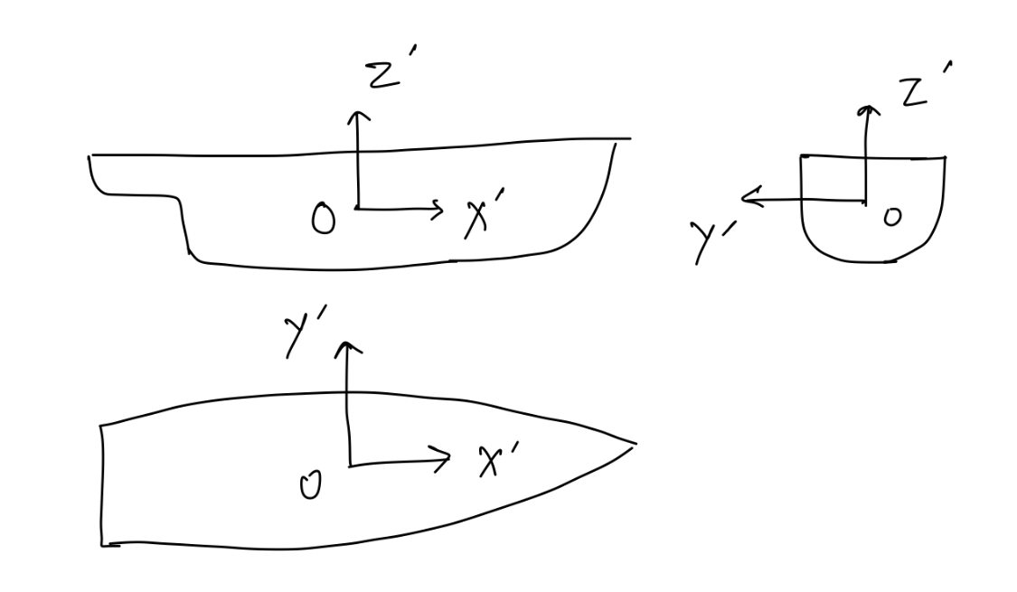
Body Coordinate System (BCS): This is a coordinate system fixed with the vehicle. As the body undergoes motion the BCS also moves with it. Thus BCS is not an inertial frame of reference. Usual convention is to choose the x-axis of BCS to be along the length of the vehicle, z-axis pointing upwards and y-axis following the right hand rule. For a ship floating in even keel, this will result in x-axis along the longitudinal direction (from aft to forward) of the ship, y-axis pointing towards port direction and z-axis pointing vertically up. The origin of the BCS may be chosen either to be at the center of gravity or a geometric point on the vessel. In general, the center of gravity of the vehicle would change depending on the vessel’s loading condition (fully loaded or ballast loaded), consumption of fuel during the voyage and due to loading or unloading of cargo at ports. Thus, it is better to choose a geometric point on the vehicle that does not change with time as the origin of BCS. The intersection of midship section, centerline and fully loaded waterline is a good choice for the origin of BCS. For underwater vehicles the geometric center of the vehicle may be chosen as the BCS origin.
The above described choice of BCS and GCS origins and their orientations are the generally used convention. One can choose the origins and frame orientations arbitrarily as long as they are maintained consistently. For ease of understanding, the convention described above will be followed in this text.
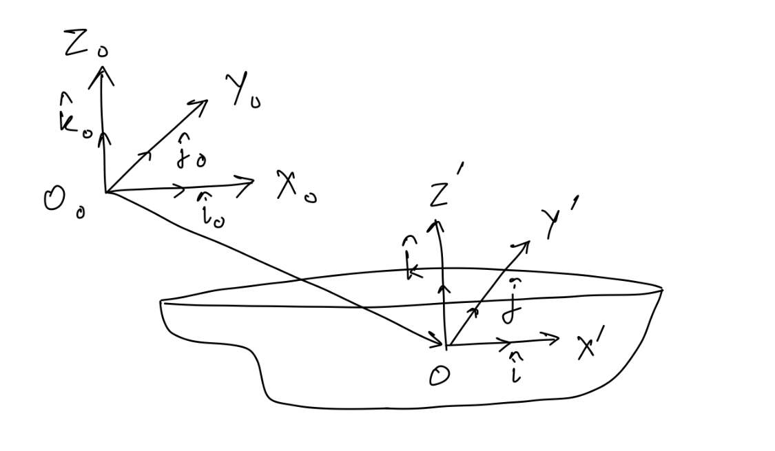
Both coordinate systems are illustrated in Figure 4.1. The origin of GCS is denoted as \(O_0\) and its axes are denoted as \(X_0Y_0Z_0\). The coordinates of a point in GCS frame will be denoted by \((x_0, y_0, z_0)\). The origin of the BCS frame is denoted by \(O'\) and its axes are denoted as \(X'Y'Z'\). The coordinates of a point expressed in BCS frame will be denoted by \((x, y, z)\).
(a) Body Coordinate System (BCS)
(b) Global Coordinate System (GCS)
Figure 4.1: Coordinate Systems
The unit vectors along the x, y and z axes of GCS are denoted as \(\hat{i}_0\), \(\hat{j}_0\) and \(\hat{k}_0\) respectively. Similarly the unit vectors along the x, y and z axes of the BCS are denoted as \(\hat{i}\), \(\hat{j}\) and \(\hat{k}\) respectively.
4.3 Pose of a Rigid Body
The pose of a rigid body can be described in terms of the above defined coordinate systems. The translation of the body is described as the position vector from the GCS origin to the BCS origin expressed in the GCS frame. In Figure 4.1 we can see that position vector of the origin of BCS in the GCS frame is given by \(\eqref{eq-gcsbcs-posvec}\).
The three parameters \(x_0\), \(y_0\) and \(z_0\) describe the translation of the body. However, as the BCS moves with the body, it may be in a different orientation as compared to the GCS at any particular instant. This means that the axes of BCS need not be parallel to the axes of GCS. Thus, the orientation also needs to be known to characterize the motion of the vehicle completely. The orientation can be described using one of the following ways:
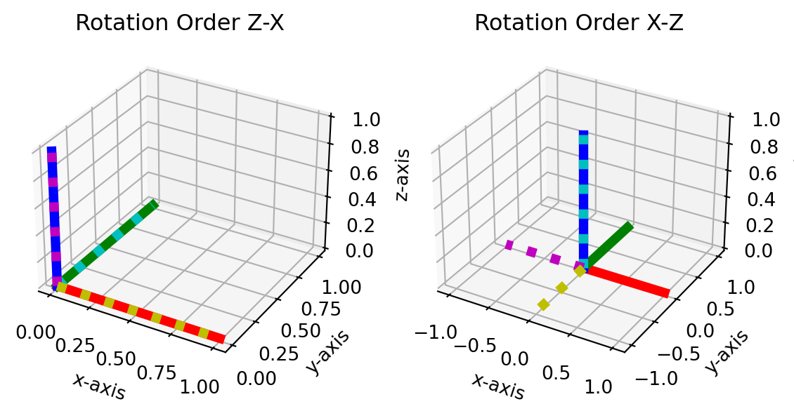
Euler angle representation: The orientation between two coordinate frames is expressed as a sequence of three rotations in a specified order. Unlike translations, rotations are not commutative and thus a specific order needs to be maintained. The non-cummutative property of rotations can be seen from Figure 4.2 where two \(90^\circ\) rotations are applied in two different orders. The first approach (left subplot) applies a \(90^\circ\) rotation about the z-axis followed by a \(90^\circ\) rotation about the new x-axis. The second approach (right subplot) interchanges the rotation order - a \(90^\circ\) rotation about the x-axis is applied first and then a \(90^\circ\) rotation is applied about the new z-axis. Note that when each rotation is taken about the body’s own new axes, the matrix of the rotation applied first stands to the left. The orientations of the new coordinate frames are completely different when the order of rotations is swapped. The Python code used to generate the results showns in Figure 4.2 is shown below, and the interactive tool at the end of this section lets you vary the axes and the angles yourself. Euler angles will be described in detail in Section 4.4.
Figure 4.2: The solid line represents the GCS orientation and the dotted line represents the BCS oreintation. For GCS, x-axis is shown in red, y-axis in green and z-axis in blue. For BCS, x-axis is shown in cyan, y-axis in magenta and z-axis in yellow. Applying 90 degrees rotation about z-axis followed by 90 degrees rotation about the new x-axis leads to the orientation shown in the left subplot. Interchanging the rotation order leads to the orientation shown in the right subplot.
Axis-angle representation: The orientation between the two coordinate frames (GCS and BCS) can be described as a single rotation about an axis of rotation that results in GCS being oriented along the BCS. The rotation is parametrized by the unit vector \(\hat{a}\) along the axis about which the rotation is performed and the magnitude of the angle of rotation \(\Theta\). This parametrization has three independent parameters. The axis being a unit vector has two independent parameters with the third parameter being constrained by the property that the vector \(\hat{a}\) is a unit vector. The third independent parameter is the angle of rotation \(\Theta\).
Quaternion: In this parametrization, the orientation between two coordinate frames (GCS and BCS) is characterized by four parameters. The parameters of a quaternion are closely related to the axis-angle representation parameters \(\Theta\) and \(\hat{a}\). The first parameter of a quaternion is \(\cos(\frac{\Theta}{2})\). The other three parameters are the components of the vector \(\sin(\frac{\Theta}{2}) \hat{a}\). The Quaternions have the primary advantage of being numerically stable, compact and efficient as compared to the other rotation formalisms. However, in contrast to the Euler angles or axis-angle representation they have one extra parameter. Quaternions have found applications in several fields including robotics, space navigation, computer vision, flight dynamics etc.
Rotation Matrix: The orientation between the two coordinate frames can also be characterized by a \(3 \times 3\) rotation matrix that has \(9\) parameters. The rotation matrix projects the vectors from one frame into another. The rotation matrix \(\boldsymbol{R}\) to project vectors from BCS to GCS is given by \(\eqref{eq-rotm-def}\). The rotation matrix to project vectors from GCS to BCS is given by the transpose of the rotation matrix denoted by \(\boldsymbol{R}^T\).
Consider a vector \(\vec{p}\) expressed in BCS. The same vector expressed in GCS \(\vec{p}_0\) is then given by premultiplying the vector \(\vec{p}\) by the rotation matrix \(\boldsymbol{R}\) as shown in \(\eqref{eq-rotm-bcs-to-gcs}\).
Some of the other formalisms of rotation in 3D space can be found here.
Each of the rotation formalisms have their own advantages and disadvantages. The rotation matrix has more parameters than any of the other formulations. Quaternions, on the other hand, represent the most compact formulation and are also numerically stable. However, they are difficult to intuitively appreciate. On the contrary, the Euler angles are most intuitive to understand and only have \(3\) parameters. The Euler angle formulation suffers from singularity at two specific orientations. This phenomenon is known as gimbal lock and will be explored more in Section 4.4.1. For marine vehicles like ships, if the order of rotation of the Euler angles is chosen well, the gimbal lock orientation is not encountered in regular operations. Thus for ships, Euler angles have become a popular approach as they are intuitive to understand.
Interactive Simulation: Order of Rotations
Figure 4.2 makes the point about non-commutativity with two static pictures. The tool below lets you make that point yourself, for any pair of axes and any pair of angles. Two identical ships start aligned with the GCS, each standing on its own tinted pedestal on which a faint copy of the fixed GCS triad is drawn. The body axes are painted on each ship (bow \(+x\) in red, port \(+y\) in green, up \(+z\) in blue) so you can watch the BCS peel away from the GCS. Drag with the mouse to orbit the view.
Both ships then perform exactly the same two rotations, in opposite orders:
the blue ship (Sequence 1) turns first by \(\alpha\) about the first axis and then by \(\beta\) about the new second axis;
the orange ship (Sequence 2) performs the same two rotations the other way round.
A dark rod marks the axis each ship is turning about at that moment. Press Play both sequences and watch step 1 and step 2 run side by side. Note that in step 2 the rod is not along a GCS axis any more: each ship turns about its own newly rotated body axis, which is precisely why the two ships part company. The readout reports the single angle through which one final orientation would have to be turned to reach the other, so a value of \(0^\circ\) means the two orders agree.
Some things worth trying:
The default setting (\(90^\circ\) about \(Z\), then \(90^\circ\) about \(X\)) reproduces Figure 4.2. The two final orientations end up \(120^\circ\) apart: the bow points along \(+y\) in Sequence 1 and along \(+z\) in Sequence 2.
Set both axes to the same letter. The disagreement collapses to \(0^\circ\): rotations about a common axis do commute, and the angles simply add.
Shrink both angles to \(5^\circ\); the disagreement falls to \(0.44^\circ\). Doubling both angles to \(10^\circ\) very nearly quadruples it, to \(1.74^\circ\) — the disagreement grows with the product of the two angles, and so is second order in the rotation angles. This is why for small angular displacements the order can be neglected and angular displacements behave like ordinary (commuting) vectors, an approximation we will lean on when linearizing the equations of motion.
Set both angles to \(180^\circ\). The disagreement returns to \(0^\circ\), so the two orders can also agree at isolated special values without the rotations commuting in general. Keeping the first angle at \(180^\circ\) and setting the second to \(90^\circ\), on the other hand, gives the worst possible case of \(180^\circ\).
Final orientations differ by 120.00°ORDER MATTERS
Sequence 1 — Z then X; bow at –Sequence 2 — X then Z; bow at –
4.4 Euler Angle Representation
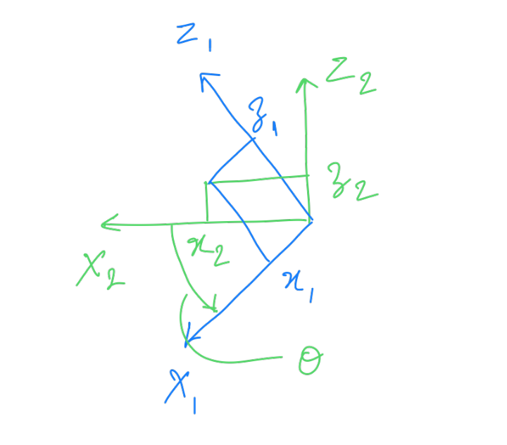
Let us consider the GCS and BCS origins to be non-coincident. In order to transform the GCS into BCS, we first translate the GCS origin to the BCS origin. This intermediate coordinate system is labelled as \(X_3Y_3Z_3\) frame. Note that \(X_3Y_3Z_3\) is parallel to GCS (\(X_0Y_0Z_0\) frame). We will assume a ZYX order of rotation from \(X_3Y_3Z_3\) frame to reach BCS (\(X'Y'Z'\) frame).
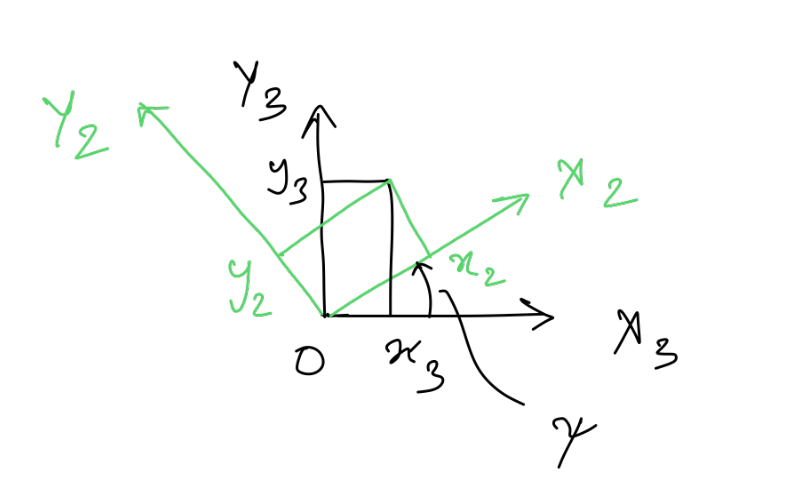
\(X_3Y_3Z_3\) is now rotated by an angle \(\psi\) about the \(Z_3\) axis to yield a new coordinate system \(X_2Y_2Z_2\) frame. Let us consider a vector \(\vec{r}_3 = [x_3 \quad y_3 \quad z_3]^T\) expressed in \(X_3Y_3Z_3\) frame. The same vector when expressed in \(X_2Y_2Z_2\) frame is denoted by \(\vec{r}_2 = [x_2 \quad y_2 \quad z_2]^T\). Since the rotation has happened along the \(Z_3\) axis, \(Z_2\) axis is coincident with \(Z_3\) axis. Therefore, the projection of the vector \(\vec{r}_3\) along \(Z_3\) axis and the projection of vector \(\vec{r}_2\) along \(Z_2\) axis is the same. Hence, \(z_2\) must be equal to \(z_3\).
Figure 4.3: Rotation from \(X_3Y_3Z_3\) to \(X_2Y_2Z_2\)
Figure 4.3 shows the rotation from \(X_3Y_3Z_3\) frame to \(X_2Y_2Z_2\) frame. Note that the \(Z_3\) and \(Z_2\) axes are coincident and are pointed out of the plane. The positive sign convention for \(\psi\) follows the right hand rule about the \(Z_3\) (or \(Z_2\)) axis and is thus denoted in the clockwise direction in Figure 4.3. From Figure 4.3 it can be seen that the \(x_3\) and \(y_3\) can be expressed in terms of \(x_2\), \(y_2\) and \(\psi\) as shown in \(\eqref{eq-z3-rotm}\) and \(\eqref{eq-z3-rotm-expanded}\).
Now \(X_2Y_2Z_2\) frame is further rotated by angle \(\theta\) about the \(Y_2\) axis to obtain the intermediate frame \(X_1Y_1Z_1\) frame. Let the \(\vec{r}_2\) vector when expressed in \(X_1Y_1Z_1\) frame be denoted by \(\vec{r}_1 = [x_1 \quad y_1 \quad z_1]^T\). Since the rotation has happened along the \(Y_2\) axis, \(Y_1\) axis is coincident with \(Y_2\) axis. Therefore, the projection of the vector \(\vec{r}_2\) along \(Y_2\) axis and the projection of vector \(\vec{r}_1\) along \(Y_1\) axis is the same. Hence, \(y_1\) must be equal to \(y_2\).
Figure 4.4: Rotation from \(X_2Y_2Z_2\) to \(X_1Y_1Z_1\)
Figure 4.4 shows the rotation from \(X_2Y_2Z_2\) frame to \(X_1Y_1Z_1\) frame. Note that the \(Y_2\) and \(Y_1\) axes are coincident and are pointed out of the plane. The positive sign convention for \(\theta\) follows the right hand rule about the \(Y_2\) (or \(Y_1\)) axis and is thus denoted in the anti-clockwise direction in Figure 4.4. From Figure 4.4 it can be seen that the \(x_2\) and \(z_2\) can be expressed in terms of \(x_1\), \(z_1\) and \(\theta\) as shown in \(\eqref{eq-y2-rotm}\) and \(\eqref{eq-y2-rotm-expanded}\).
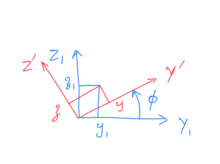
Now \(X_1Y_1Z_1\) frame is finally rotated by angle \(\phi\) about the \(X_1\) axis to obtain the BCS frame \(X'Y'Z'\). Let the \(\vec{r}_1\) vector when expressed in BCS frame be denoted by \(\vec{r} = [x \quad y \quad z]^T\). Since the rotation has happened along the \(X_1\) axis, \(X'\) axis is coincident with \(X_1\) axis. Therefore, the projection of the vector \(\vec{r}_1\) along \(X_1\) axis and the projection of vector \(\vec{r}\) along \(X'\) axes is the same. Hence, \(x\) must be equal to \(x_1\).
Figure 4.5: Rotation from \(X_1Y_1Z_1\) to \(X'Y'Z' (BCS)\)
Figure 4.5 shows the rotation from \(X_1Y_1Z_1\) frame to \(X'Y'Z'\) frame (BCS). Note that the \(X_1\) and \(X'\) axes are coincident and are pointed out of the plane. The positive sign convention for \(\phi\) follows the right hand rule about the \(X_1\) (or \(X'\)) axis and is thus clockwise in Figure 4.5. From Figure 4.5 it can be seen that \(y_1\) and \(z_1\) can be expressed in terms of \(y\), \(z\) and \(\phi\) as shown in \(\eqref{eq-x1-rotm}\) and \(\eqref{eq-x1-rotm-expanded}\).
By combining \(\eqref{eq-z3-rotm}\), \(\eqref{eq-y2-rotm}\) and \(\eqref{eq-x1-rotm}\) the vector \(\vec{r}_3\) can be expressed in terms of the vector \(\vec{r}\) as shown in \(\eqref{eq-rotm-fomulation}\).
where \(s_1 = \sin(\phi)\), \(c_1 = \cos(\phi)\), \(s_2 = \sin(\theta)\), \(c_2=\cos(\theta)\), \(s_3 = \sin(\psi)\) and \(c_3 = \cos(\psi)\). The rotation matrix \(\boldsymbol{R}\) transforms any vector in the BCS to the GCS. The rotation matrix is defined by the Euler angles \(\phi\), \(\theta\) and \(\psi\). Rotation matrices are orthogonal matrices, which means that the transpose of the matrix is its inverse. Mathematically it can be expressed as shown in \(\eqref{eq-rotm-orthogonal}\).
In this case the rotation matrix becomes degenerate. This means that unique mapping is lost at this point. Several combinations of \(\phi\) and \(\psi\) that have the same value of \(\phi - \psi\) will lead to the same rotation matrix. For example, \((\phi, \theta, \psi) = (10^\circ, 90^\circ, 5^\circ)\) and \((\phi, \theta, \psi) = (5^\circ, 90^\circ, 0^\circ)\) will lead to the same rotation matrix. This phenomenon is called gimbal lock. It is called a gimbal lock as in this representation there is no way to roll the vehicle (for the ZYX rotation order) without pitching it out of the gimbal lock position.
For Euler angle formulation based on ZYX order of rotation, gimbal lock will happen when \(\theta = \frac{n\pi}{2}\) for \(n=\pm1, \pm2, ...\) Note that this phenomenon happens for all Euler angle formulations regardless of the order of rotation. Whenever the second rotation results in the first and the third axes of rotations being coincident, this degeneracy will manifest.
Common Confusion
The common confusion is - does physically the rigid body experience any problem when passing through this degenerate point of \(\theta = \pm \frac{\pi}{2}\)?
Remember that the Euler angle notation is our way of representing the pose of the rigid body. The degenracy is in our way of representing the orientation and not with the physical world. So when physically the rigid body moves through a gimbal lock orientation, our representation of orientation will result in a funny looking motion. Quaternions based representation of oreintation does not suffer from the problem of gimbal lock and hence has been widely adopted in the fields of robotics, computer vision, computer graphics, flight dynamics etc.
Check out this YouTube video on Gimbal lock for better visualization.
Interactive Simulation
Use the tool below to explore gimbal lock directly. The ship is mounted inside a mechanical three-ring gimbal that realizes the ZYX rotation order: the outer blue ring rotates about the fixed vertical yaw axis (\(\psi\)), the middle green ring rotates about the pitch axis (\(\theta\)) carried by the blue ring, and the inner red ring rotates about the roll axis (\(\phi\)) carried by the green ring. The body axes of the ship are drawn on it (bow \(+x\) in red, port \(+y\) in green, up \(+z\) in blue) and the fixed GCS triad is shown in the corner. Drag with the mouse to orbit the view.
Press Drive to gimbal lock to animate the pitch angle to \(\theta = 90^\circ\) and watch the red roll axis swing into alignment with the blue yaw axis. Then press Wiggle \(\psi\) and Wiggle \(\phi\) in turn: away from gimbal lock they produce clearly different motions of the ship, but at \(\theta = 90^\circ\) they rotate the ship about the same physical axis — one degree of freedom has been lost, exactly as \(\eqref{eq-rotm-gimbal-lock}\) predicts (only \(\phi - \psi\) matters). The readouts track the angle between the roll and yaw axes and \(\det(\boldsymbol{J}_2^{-1}) = \cos\theta\), which vanishes at the singularity of \(\eqref{eq-kinematics-rotation}\).
There exist 12 different possible rotation orders when defining Euler angles. These can be separated into two groups:
Proper Euler Angles (ZXZ, XYX, YZY, ZYZ, XZX and YXY)
Tait-Bryan Angles (XYZ, ZXY, YZX, XZY, ZYX and YZX)
The Tait-Bryan angles represent rotations about three distinct axes while proper Euler angles use the same axes for the first and third elemental rotations. For marine vehicles, the common rotation order used is ZYX order. Notice that for this choice of rotation order, the gimbal lock orientations occur when the vehicle pitches up or down by \(90^{\circ}\). As marine vehicles like ships and underwater vehicles do not pitch by large angles during regular operations, this representation serves well to describe orientations uniquely. Unless specified explicitly, this text will assume a ZYX order of rotation when referring to Euler angles.
4.4.2 Equivalence with the Axis-Angle Representation
The Euler angles and the axis-angle parameters are two different parametrizations of the very same object - the rotation matrix \(\boldsymbol{R}\) that carries the GCS orientation onto the BCS orientation. Whatever three Euler angles \((\phi, \theta, \psi)\) are chosen, the resulting \(\boldsymbol{R}\) of \(\eqref{eq-rotm-expansion}\) can always be reached instead by a single rotation of some angle \(\Theta\) about some fixed unit vector \(\hat{a}\). This is Euler’s rotation theorem, and it is what guarantees that the axis-angle representation is complete.
The axis \(\hat{a}\) and the angle \(\Theta\) can be recovered from \(\boldsymbol{R}\) directly. Since \(\hat{a}\) is unchanged by the rotation, it is the eigenvector of \(\boldsymbol{R}\) belonging to the eigenvalue \(1\):
This has an important consequence that is easy to miss: because \(\hat{a}\) is left alone by the transformation, its components are the same whether it is expressed in the GCS or in the BCS. It is the one direction on which the two frames agree. The angle follows from the trace, which is invariant under a change of frame:
Going the other way, the rotation matrix is rebuilt from \(\hat{a}\) and \(\Theta\) by Rodrigues’ rotation formula, in which \(\boldsymbol{S}(\hat{a})\) is the skew-symmetric matrix representing the cross product \(\hat{a} \times (\cdot)\):
The tool below shows the two parametrizations arriving at the same place. Both ships start aligned with the GCS. The blue ship takes the Euler route of Section 4.4: yaw \(\psi\) about \(Z_3\), then pitch \(\theta\) about the new \(Y_2\), then roll \(\phi\) about the new \(X_1\) — three separate turns about three different axes, each one about an axis that the previous turn has already moved. The orange ship takes the axis-angle route: one single, steady turn of \(\Theta\) about the purple axis \(\hat{a}\). Press Play both routes and watch them land in exactly the same attitude.
Notice that the purple axis is drawn identically on both pedestals and never moves — it is fixed in the GCS, and by \(\eqref{eq-axis-eigenvector}\) it has the same three components in the BCS as well. At the end of the animation, the blue ship’s body axes are arranged about that rod in precisely the same way as the orange ship’s.
The two matrices printed below the view are computed by genuinely independent routes: the left one is \(\eqref{eq-rotm-expansion}\) evaluated from \((\phi, \theta, \psi)\), and the right one is Rodrigues’ formula \(\eqref{eq-rodrigues}\) evaluated from the extracted \((\hat{a}, \Theta)\). The reported largest element-wise difference between them stays at the level of machine round-off, which is the numerical statement of the equivalence.
Some things worth trying:
At the default setting \((\phi, \theta, \psi) = (30^\circ, 45^\circ, 60^\circ)\) the equivalent single rotation is \(\Theta = 69.36^\circ\) about \(\hat{a} = (0.0391,\ 0.7728,\ 0.6335)\). Move any one slider and watch both change: there is no simple correspondence, as a change in a single Euler angle generally tilts the equivalent axis and alters the equivalent angle.
Set \(\phi = \theta = 0\) and vary \(\psi\) alone. The equivalent axis snaps to \(\hat{a} = (0, 0, 1)\) with \(\Theta = \psi\): with only one rotation active, the two representations trivially coincide. (For negative \(\psi\) the tool reports \(\hat{a} = (0,0,-1)\) and \(\Theta = |\psi|\), since it always chooses the representation with \(0 \leq \Theta \leq 180^\circ\).)
Set \(\theta = 90^\circ\) and then vary \(\phi\) and \(\psi\) keeping \(\phi - \psi\) fixed. The Euler angles change but the axis, the angle and both matrices do not — this is the gimbal lock degeneracy of Section 4.4.1 seen from the other side. The axis-angle parameters remain perfectly well behaved throughout, which is exactly why axis-angle and quaternion representations do not suffer from gimbal lock.
Drive all three angles up and watch \(\Theta\) approach \(180^\circ\). This is the one orientation at which the axis-angle representation has its own awkwardness: at \(\Theta = 180^\circ\) the axes \(\hat{a}\) and \(-\hat{a}\) describe the same rotation, so the parametrization is two-to-one there.
Let the Euler angles be defined as a vector as shown in \(\eqref{eq-euler-angles}\). Note that this vector does not physically represent any geometric quantity. Remember that each of the angles sequentially denote the rotations from GCS through the intermediate frames to the BCS.
Let the translational velocity of the vehicle expressed in BCS be defined as shown in \(\eqref{eq-bcs-vel}\). Note that the vector notation and matrix notations are used interchangably. This interchange of notations will be useful later when we would want to express cross product of vectors in terms of matrix muliplications.
\[\begin{align}
\vec{v} = \{\nu_1\} = \begin{bmatrix} u & v & w\end{bmatrix}^T = u \hat{i} + v\hat{j} + w\hat{k}
\label{eq-bcs-vel}
\end{align}\]
Similarly the angular velocity of the vehicle in BCS is defined as shown in \(\eqref{eq-bcs-ang-vel}\).
\[\begin{align}
\vec{\omega} = \{\nu_2\} = \begin{bmatrix} p & q & r\end{bmatrix}^T = p \hat{i} + q\hat{j} + r\hat{k}
\label{eq-bcs-ang-vel}
\end{align}\]
The total velocity vector \(\{\nu\}\) is defined as the concatenation of \(\{\nu_1\}\) and \(\{\nu_2\}\) as shown in \(\eqref{eq-vel-vec}\).
\[\begin{align}
\{\nu\} = \begin{bmatrix}\{\nu_1\}^T & \{\nu_2\}^T \end{bmatrix}^T = \begin{bmatrix} u & v & w & p & q & r \end{bmatrix}^T
\label{eq-vel-vec}
\end{align}\]
Now \(\frac{d}{dt}\{\eta\} = \{\dot{\eta}_1\}\) represents the time derivative of the position vector of BCS origin expressed in the GCS. Since GCS is an inertial frame of reference, \(\{\dot{\eta}_1\}\) is the translational velocity of the BCS origin with respect to GCS. The translational velocity of BCS origin expressed in BCS is given by \(\{\nu_1\}\). These two vectors are related through \(\eqref{eq-kinematics-translation}\).
Why \(\{\nu_1\} \neq 0\)? \(\{\nu_1\}\) represents the velocity of the body in BCS frame and if the BCS is moving with the body, then the relative velocity of the body with respect to BCS should be zero?
Note that \(\{\nu_1\}\) represents the velocity of the BCS orgin with respect to GCS origin expressed in BCS. It is NOT the velocity of the BCS origin with respect to BCS origin expressed in BCS. The velocity of the BCS origin with respect to BCS origin expressed in BCS will definitely be zero!
The angular velocity \(\{\nu_2\}\) and the derivative of the Euler angles \(\{\dot{\eta}_2\}\) can also be related as was seen for the translational velocity in \(\eqref{eq-kinematics-translation}\). However, the relation is not simply through a rotation matrix!
The Euler angles sequentially denote the rotations from GCS through the intermediate frames to the BCS. Thus each Euler angle is defined with respect to different frames of reference and the contribution of each Euler rate to the total angular velocity needs to be computed separately. The total angular velocity of the body is the sum of angular velocities due to each of the Euler rates.
Let us consider the contribution to angular velocity due to \(\dot{\phi}\). The angle \(\phi\) is defined about the \(X'\) axis (or equivalently \(X_1\) axis). Since \(X'\) axis is one of the cardinal axes of the BCS, the contribution to angular velocity is given by \(\eqref{eq-ang-vel-comp-phi}\).
As \(\theta\) is defined about the \(Y_1\) axis (or equivalently \(Y_2\) axis), the contribution to angular velocity due to \(\dot{\theta}\) is given by \(\eqref{eq-ang-vel-comp-theta}\). Note that Euler rate \(\dot{\theta}\) is the angular velocity in the \(X_1Y_1Z_1\) frame and needs to be transformed into BCS. Therefore, it is premultiplied by \(\boldsymbol{R}_{x,\phi}^T\).
As \(\psi\) is defined about the \(Z_2\) axis (or equivalently \(Z_3\) axis), the contribution to angular velocity due to \(\dot{\psi}\) is given by \(\eqref{eq-ang-vel-comp-psi}\). Note that Euler rate \(\dot{\psi}\) is the angular velocity in the \(X_2Y_2Z_2\) frame and needs to be transformed into BCS. Therefore, it is premultiplied by \(\boldsymbol{R}_{x,\phi}^T\boldsymbol{R}_{y,\theta}^T\).
Thus combining \(\eqref{eq-ang-vel-comp-phi}\), \(\eqref{eq-ang-vel-comp-theta}\) and \(\eqref{eq-ang-vel-comp-psi}\) the total angular velocity is given by \(\eqref{eq-ang-vel-comp}\) and \(\eqref{eq-ang-vel}\).
Thus the Euler rates are given by \(\eqref{eq-kinematics-rotation}\). Note that \(\boldsymbol{J}_2\) matrix becomes singular when gimbal lock occurs (\(\theta=\frac{n\pi}{2}\) for \(n=\pm 1, \pm 2, ...\)).
In a compact form this can be written as shown in \(\eqref{eq-kinematics-compact}\). This matrix differential equation represents the kinematics of a rigid body.
If the amplitude of motion and velocities are assumed to be small quantities, then the kinematic equations can be linearized as \(\eqref{eq-kinematics-linear}\).
Note that so far the discussion has been centered around the motion itself and not on the cause of the motion. In the next chapter the dynamic equation of motion that describe the cause of the motion will be discussed.
4.7 Exercises
Throughout, the GCS is the East–North–Up frame of Chapter 4 and the BCS has \(x\) along the bow, \(y\) to port and \(z\) up. All Euler angles follow the ZYX order of Section 4.4, so that \(\boldsymbol{R} = \boldsymbol{R}_{z,\psi}\boldsymbol{R}_{y,\theta}\boldsymbol{R}_{x,\phi}\) carries a vector from the BCS to the GCS. The heading \(\psi\) is measured about \(Z_0\) from the \(X_0\) axis by the right hand rule, not from North as a navigator would quote it.
Every problem below can be solved with the results of this chapter alone — the definition \(\eqref{eq-rotm-def}\) of the rotation matrix, the elemental matrices \(\eqref{eq-z3-rotm-expanded}\), \(\eqref{eq-y2-rotm-expanded}\) and \(\eqref{eq-x1-rotm-expanded}\), the assembled matrix \(\eqref{eq-rotm-expansion}\), the orthogonality property \(\eqref{eq-rotm-orthogonal}\), the gimbal lock condition of Section 4.4.1 and the kinematic equations \(\eqref{eq-kinematics-translation}\), \(\eqref{eq-ang-vel}\) and \(\eqref{eq-kinematics-rotation}\) — together with elementary vector algebra. The axis–angle and quaternion parametrizations are not required anywhere and should not be used. No hydrodynamics, wave theory or knowledge of the forces causing the motion is needed: wherever a velocity, a rate or an angle is required it is given to you.
One consequence of the book’s conventions is worth stating before you start, because it catches almost everyone. With \(z\) up and \(y\) to port, the bow direction is the first column of \(\eqref{eq-rotm-expansion}\), whose vertical component is \(-\sin\theta\). A positive pitch \(\theta\) therefore drives the bow downwards, and a vehicle descending under way carries \(\theta > 0\). This is the opposite sense to the aeronautical convention, in which a positive pitch is nose-up, and the difference is entirely due to the choice of an \(z\)-up rather than a \(z\)-down global frame.
Several problems ask you to derive a result before using it numerically; the derivation carries most of the marks. Principal dimensions are representative rather than exact and serve only to give the numbers a realistic scale. Use \(g = 9.81\) m/s\(^2\).
The vessels and the frames used in these exercises
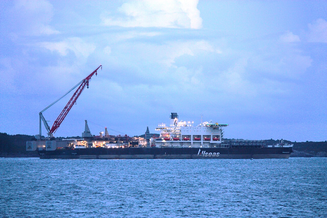
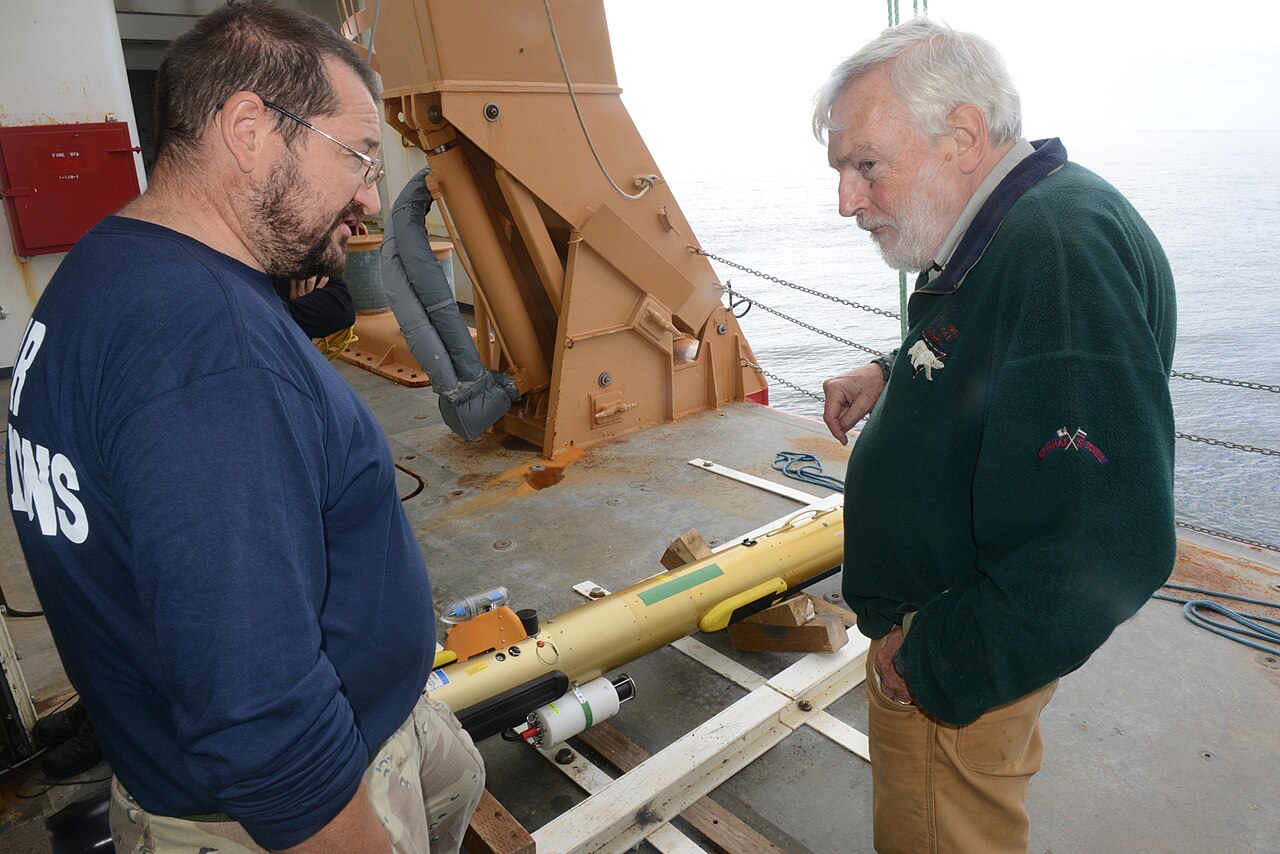
The problems below are about three kinds of vehicle. Figure 4.6 shows two of them. Problems 1, 3 and 5 concern heavy-lift and installation work, where a vessel’s attitude has to be known to a fraction of a degree because a topside weighing tens of thousands of tonnes must be set down on a jacket without touching its legs. Problems 6, 7 and 8 concern a torpedo-shaped autonomous underwater vehicle, which has no vertical thruster at all: it changes depth by pitching its whole body and flying, which is why the coupling between its attitude and its velocity is the heart of those problems.
(a) A heavy-lift and installation vessel. Placing or removing a complete topside is a centimetre-and-fraction-of-a-degree operation, and every quantity in it is quoted relative to a frame that must be stated unambiguously — the subject of Problems 1, 3 and 5.
(b) A torpedo-shaped autonomous underwater vehicle on deck before launch. Its only actuators are a propeller on the body \(x\) axis and control surfaces that set the attitude, so depth is changed by pitching the hull — the situation of Problems 6, 7 and 8.
Figure 4.6: Two of the vehicle types used in the exercises of this chapter. Image credits: (a) Cavernia, CC0; (b) U.S. Coast Guard, Petty Officer 1st Class Shawn Eggert, public domain. Both are hosted on Wikimedia Commons.
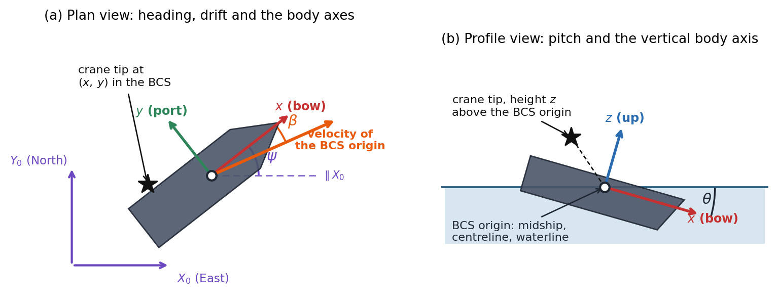
Figure 4.7 fixes the notation. Every angle, axis and offset used in the problems appears on it once, drawn in the book’s conventions: the GCS is East-North-Up, the body \(x\) axis runs along the bow, \(y\) to port and \(z\) up, and the BCS origin sits at midship on the centreline at the waterline. Note in particular that the heading \(\psi\) is measured at the BCS origin against a line parallel to \(X_0\), and that the velocity of the origin need not lie along the centreline — the angle between them is the drift angle used in Problems 6 and 10.
Figure 4.7: The frames, angles and offsets used throughout these exercises. (a) Plan view, looking down: the fixed GCS axes, the body axes carried by the vessel, the heading \(\psi\), and the drift angle \(\beta\) between the centreline and the velocity of the BCS origin. (b) Profile view: the pitch \(\theta\) and the body \(z\) axis. The star marks a point fixed in the vessel, such as the crane tip of Problem 2, whose body-frame coordinates are \((x, y, z)\). Angles are drawn larger than they would ever be in service.
Reading a platform’s orientation off a survey. During a jacket installation the orientation of a heavy-lift vessel is fixed by a survey that reports the directions of two of the vessel’s body axes, expressed in the GCS: \[\hat{i} = [0.8147,\ 0.5704,\ 0.1045]^T, \qquad \hat{j} = [-0.5788,\ 0.7888,\ 0.2068]^T\]
Starting from the definition \(\eqref{eq-rotm-def}\), show that the columns of \(\boldsymbol{R}\) are the BCS unit vectors \(\hat{i}\), \(\hat{j}\), \(\hat{k}\) expressed in the GCS, while the rows of \(\boldsymbol{R}\) are the GCS unit vectors \(\hat{i}_0\), \(\hat{j}_0\), \(\hat{k}_0\) expressed in the BCS. Which of these two statements makes \(\boldsymbol{R}^T\) the GCS \(\to\) BCS transformation?
Verify that the two reported vectors are of unit length and mutually orthogonal to within the quoted precision. Construct the missing third body axis and assemble \(\boldsymbol{R}\). Explain why the right handedness of the BCS is what forces your choice of sign, and state what a survey with \(\hat{k} = -\hat{i}\times\hat{j}\) would imply about the reported data.
By comparing your matrix with \(\eqref{eq-rotm-expansion}\), derive general expressions for \(\phi\), \(\theta\) and \(\psi\) in terms of the elements \(R_{ij}\), and evaluate them. Explain why the third row and first column are the natural places to look, and why a four-quadrant \(\operatorname{atan2}\) is needed for \(\phi\) and \(\psi\) but not for \(\theta\).
Show algebraically, using \(\eqref{eq-rotm-expansion}\), that the triple \((\phi + 180^\circ,\ 180^\circ - \theta,\ \psi + 180^\circ)\) produces exactly the same \(\boldsymbol{R}\) as \((\phi, \theta, \psi)\). Evaluate this second solution for the surveyed matrix, and explain how restricting \(\theta\) to \([-90^\circ, 90^\circ]\) removes the ambiguity. Which of the two solutions would a naive \(\theta = \arcsin(-R_{31})\) always return, and why?
A second survey crew mounts its reference frame with \(x\) pointing aft and \(y\) to starboard — that is, their BCS is the vessel’s BCS rotated by \(180^\circ\) about its own \(z\) axis. Show that their rotation matrix is \(\boldsymbol{R}\boldsymbol{R}_{z,180^\circ}\), prove that their Euler angles are exactly \((-\phi,\ -\theta,\ \psi - 180^\circ)\), and evaluate them. A colleague concludes that the vessel is now pitching and rolling the other way. Is anything physical different?
Where the crane tip actually goes. An FPSO carries a deck crane whose tip, when the boom is slewed out on the port quarter, sits at \[\vec{r} = [-45,\ 28,\ 30]^T \text{ m}\] in the BCS, the BCS origin being at the intersection of midship, centreline and the loaded waterline. At one instant the vessel’s pose is \(\{\eta_1\} = [120,\ -340,\ 1.2]^T\) m and \(\{\eta_2\} = (\phi, \theta, \psi) = (4^\circ,\ 2^\circ,\ 30^\circ)\).
Write down the GCS position of the crane tip in terms of \(\{\eta_1\}\), \(\boldsymbol{R}\) and \(\vec{r}\), justify it in one sentence, and evaluate it.
Show from \(\eqref{eq-rotm-expansion}\) that the vertical GCS coordinate of any point fixed in the vessel is independent of the heading \(\psi\), exactly and not merely to first order. Which structural feature of \(\boldsymbol{R}_{z,\psi}\) is responsible?
Expand \(\eqref{eq-rotm-expansion}\) to first order in the three angles to show that \[\boldsymbol{R} \approx \boldsymbol{I} + \boldsymbol{S}, \qquad \boldsymbol{S} = \begin{bmatrix} 0 & -\psi & \theta \\ \psi & 0 & -\phi \\ -\theta & \phi & 0\end{bmatrix}\] and hence that the displacement of a point \(\vec{r}\) relative to the BCS origin is \(\boldsymbol{S}\vec{r}\). Deduce that the vertical component is \(\delta z \approx \phi y - \theta x\), and note which coordinate of \(\vec{r}\) is absent from it.
The vessel oscillates with roll amplitude \(4^\circ\), pitch amplitude \(2^\circ\) and heave amplitude \(1.2\) m, all in phase. Compute the amplitude of the vertical motion of the crane tip from the approximation of part (c) and from the exact matrix, and compare both with the heave amplitude alone. By what factor is the motion at the tip amplified, and what is the error committed by linearizing?
Find the locus of points on the deck at which the first-order vertical motion vanishes for these amplitudes, and describe it geometrically. Explain why this “quiet line” rotates as the ratio of roll to pitch amplitude changes with sea state, and why that makes it useless as a permanent siting rule for motion-sensitive equipment.
Two conventions, one platform. A motion reference unit on a heavy-lift vessel reports \((\phi, \theta, \psi) = (8^\circ,\ 5^\circ,\ 40^\circ)\). The vendor’s manual defines these angles in the XYZ order, that is \(\boldsymbol{R}_{XYZ} = \boldsymbol{R}_{x,\phi}\boldsymbol{R}_{y,\theta}\boldsymbol{R}_{z,\psi}\), whereas the lift-analysis software assumes the ZYX order \(\eqref{eq-rotm-fomulation}\) of this chapter.
Compute both matrices. Extract the bow direction \(\hat{i}\) in the GCS from each, and find the angle between the two bow directions. Do the same for the mast direction \(\hat{k}\).
Determine the ZYX angles that describe the orientation the vendor actually intended, and hence state the roll, pitch and heading errors committed by feeding the vendor’s three numbers straight into the software.
The lift plan is rejected if the heading is wrong by more than \(1^\circ\). Would this error be caught by a heading check alone? Comment on why an error of this kind is easy to miss in practice.
Show that to first order in the angles every rotation order gives the same matrix \(\boldsymbol{I} + \boldsymbol{S}\) of Problem 2(c), so that the two conventions can only differ at second order. Verify this by repeating part (a) with all three angles divided by \(10\), and confirm that the angle between the two bow directions falls by roughly a factor of \(100\).
Show that if any two of the three angles are zero, all rotation orders agree exactly. Use this to explain why a convention error can lie dormant through an entire calm-water commissioning trial and only appear once the vessel is working in a seaway.
What a levelling sensor can and cannot see. A three-axis accelerometer is bolted to the deck of a moored platform, aligned with the BCS. The platform is at rest, so the only acceleration the instrument senses is that due to gravity, which in the GCS is \([0,\ 0,\ -g]^T\). The instrument reads \[\vec{a} = [0.8550,\ -1.2925,\ -9.6868]^T \text{ m/s}^2\]
Show that the reading must be \(\vec{a} = \boldsymbol{R}^T[0,\ 0,\ -g]^T\), and hence, using \(\eqref{eq-rotm-expansion}\), that \[\vec{a} = g\,[\sin\theta,\ -\sin\phi\cos\theta,\ -\cos\phi\cos\theta]^T\] Confirm that \(|\vec{a}| = g\) for every orientation, and say which property of \(\boldsymbol{R}\) guarantees it.
Invert these relations to obtain \(\theta\) and \(\phi\) from the reading, and evaluate them. Then show that \(\psi\)cannot be obtained from this measurement at any orientation, and explain the reason in terms of the order of the ZYX rotations and the direction of gravity.
Verify your answer by reconstructing \(\vec{a}\) from the recovered angles.
Differentiate the relation for \(\theta\) to show that \(\mathrm{d}\theta/\mathrm{d}a_x = 1/(g\cos\theta)\). A cheap accelerometer has a bias of \(0.02\) m/s\(^2\) on each channel. Compute the resulting pitch error at \(\theta = 0^\circ\), \(60^\circ\) and \(85^\circ\), and comment on the trend.
Show that at \(\theta = \pm 90^\circ\) the reading becomes \(\vec{a} = \pm g\,[1,\ 0,\ 0]^T\)whatever the value of \(\phi\), so that roll joins heading in being unmeasurable. Relate this to Section 4.4.1, and state what additional sensor a vessel must carry to determine the orientation completely.
Float-over: the relative orientation of two bodies. In a float-over installation a barge carries the topsides between the legs of a jacket and lowers them onto it. What matters for mating is not the attitude of either body in the GCS, but the attitude of the barge relative to the jacket. Just before mating, surveys give
The mating tolerance requires relative roll and relative pitch each below \(0.5^\circ\) and relative heading below \(1.0^\circ\).
Let \(\boldsymbol{R}_J\) and \(\boldsymbol{R}_B\) carry vectors from the jacket frame and the barge frame respectively into the GCS. Derive the matrix that carries a vector from the barge frame into the jacket frame, and verify from \(\eqref{eq-rotm-orthogonal}\) that it is itself a rotation matrix.
Evaluate this relative matrix and extract its ZYX Euler angles.
A junior engineer computes the relative attitude as the difference of the two sets of Euler angles. Evaluate that difference, compare it with the exact answer of part (b), and quantify the discrepancy in each channel.
Show that the difference rule is correct to first order but wrong at second order, and confirm the size of the discrepancy against the products of the angles involved. Express the largest discrepancy as a percentage of the tightest tolerance and comment on whether the shortcut is acceptable here.
The barge is to be re-ballasted to bring the relative pitch to zero without altering its heading or its roll. Determine the required \(\theta_B\), and state whether the naive answer \(\theta_B = \theta_J\) is adequate.
Speed over ground, drift and the climb of a trimmed vehicle. A survey vessel has body-frame velocity components \(u = 6.2\) m/s, \(v = -0.9\) m/s, \(w = 0.15\) m/s at an instant when its pose angles are \((\phi, \theta, \psi) = (-6^\circ,\ 1.5^\circ,\ 62^\circ)\).
Compute \(\{\dot{\eta}_1\}\) from \(\eqref{eq-kinematics-translation}\). Define the course over ground as \(\chi = \operatorname{atan2}(\dot{y}_0, \dot{x}_0)\) and evaluate it.
Show that when \(\phi = \theta = 0\) the course is exactly \(\chi = \psi + \operatorname{atan2}(v, u)\), so that the difference between course and heading is precisely the drift (sideslip) angle. Evaluate this idealized course for the given \(u\) and \(v\), and compare it with the exact value from part (a). How large is the error introduced by ignoring the \(6^\circ\) of heel?
Prove from \(\eqref{eq-rotm-orthogonal}\) that \(|\{\dot{\eta}_1\}| = |\{\nu_1\}|\) for every orientation, and verify numerically. Then compute the horizontal speed made good and explain why it is smaller.
Show from the third row of \(\eqref{eq-rotm-expansion}\) that \[\dot{z}_0 = -u\sin\theta + v\sin\phi\cos\theta + w\cos\phi\cos\theta\] and hence that a vehicle with no heave velocity in body axes still changes altitude whenever it is trimmed and moving ahead. Evaluate \(\dot{z}_0\) for the given data with \(w\) set to zero.
An AUV runs at \(2.0\) m/s along its own \(x\) axis with \(v = w = 0\) and no heel. Derive its rate of descent as a function of pitch and evaluate it at \(\theta = 10^\circ\) (bow down, by the sign convention noted at the head of these exercises). How long does it take to reach \(150\) m depth, and what horizontal distance does it cover doing so? Comment on why a vehicle that is nominally “swimming forwards” is in fact the standard way to change depth.
Euler rates are not an angular velocity. A survey AUV is flying a steady helical descent, holding a constant bank \(\phi = 15^\circ\) and a constant bow-down pitch \(\theta = 20^\circ\) while its heading changes at the constant rate \(\dot{\psi} = 0.05\) rad/s.
Compute the body-frame angular velocity \(\{\nu_2\} = [p, q, r]^T\) from \(\eqref{eq-ang-vel}\). All three components are non-zero even though only one Euler angle is changing — explain why in terms of the axis about which \(\dot{\psi}\) acts.
Show that \(r = \dot{\psi}\cos\phi\cos\theta\) whenever \(\dot{\phi} = \dot{\theta} = 0\), so a yaw-axis rate gyro always under-reads the turn rate of a banked or pitched vehicle. Evaluate the shortfall here, and compute the heading error accumulated if \(r\) is naively integrated as \(\dot{\psi}\) over a five-minute descent.
At a later instant, while the attitude is momentarily the same \((\phi, \theta) = (15^\circ,\ 20^\circ)\), the instruments record \(p = 0.030\), \(q = 0.012\), \(r = -0.045\) rad/s. Compute the Euler rates from \(\eqref{eq-kinematics-rotation}\).
For the rates of part (c) compute \(|\{\dot{\eta}_2\}|\) and \(|\{\nu_2\}|\) and show that they differ. Then show that for the single-rate case of part (a) they agree exactly, and explain what distinguishes the two situations.
The columns of \(\boldsymbol{J}_2^{-1}\) are the three unit vectors about which \(\dot{\phi}\), \(\dot{\theta}\) and \(\dot{\psi}\) act, expressed in the BCS. Write them down from \(\eqref{eq-ang-vel}\), verify that each is of unit length, and show that while the \(\dot{\phi}\) and \(\dot{\theta}\) axes are perpendicular, and the \(\dot{\theta}\) and \(\dot{\psi}\) axes are perpendicular, the angle between the \(\dot{\phi}\) and \(\dot{\psi}\) axes is \(90^\circ + \theta\). Evaluate it here. This non-orthogonality is the whole reason \(\{\eta_2\}\) is not a vector: explain why, and predict from the formula what happens at \(\theta = 90^\circ\).
Gimbal lock in a hovering AUV. A hover-capable inspection AUV is commanded to pitch nose-up through the vertical so as to inspect the underside of a platform deck. Its control software carries the orientation as ZYX Euler angles.
Verify \(\eqref{eq-rotm-gimbal-lock}\) by evaluating \(\boldsymbol{R}\) at \((\phi, \theta, \psi) = (35^\circ,\ 90^\circ,\ 20^\circ)\) and at \((50^\circ,\ 90^\circ,\ 35^\circ)\), and comment on the result. Give a third, quite different pair \((\phi, \psi)\) producing the same matrix.
With the body rates held at \([p, q, r] = [0.02,\ 0.05,\ 0.01]\) rad/s and \(\phi = 35^\circ\), tabulate the Euler rates from \(\eqref{eq-kinematics-rotation}\) at \(\theta = 60^\circ\), \(80^\circ\), \(88^\circ\), \(89.5^\circ\) and \(89.9^\circ\). Identify which rates diverge and confirm that they grow as \(1/\cos\theta\).
Compute \(|\{\nu_2\}|\) at each of those pitch angles. What does the contrast with part (b) tell you about where the difficulty actually lies?
Evaluate \(\boldsymbol{J}_2^{-1}\) at \(\theta = 90^\circ\) and find a non-zero \(\{\dot{\eta}_2\}\) for which \(\{\nu_2\} = 0\). Interpret this vector physically, and reconcile it with your answer to part (a).
Show that at \(\theta = 90^\circ\) the columns of \(\boldsymbol{J}_2^{-1}\) span only a two-dimensional space, and find the body-axis direction of angular velocity that no choice of Euler rates can produce. Is the AUV physically unable to rotate that way? State the practical remedy, and explain why a ZYX order is nevertheless the right choice for a conventional ship.
When may the kinematics be linearized? Almost the whole of seakeeping theory replaces \(\eqref{eq-kinematics-compact}\) by \(\{\dot{\eta}\} \approx \{\nu\}\). This problem establishes what that costs.
Using the first-order expansions of Problem 2(c), show that \(\boldsymbol{R} = \boldsymbol{I} + \boldsymbol{S} + O(2)\) and, from \(\eqref{eq-kinematics-rotation}\), that \[\boldsymbol{J}_2 = \boldsymbol{I} + \boldsymbol{T} + O(2), \qquad \boldsymbol{T} = \begin{bmatrix} 0 & 0 & \theta \\ 0 & 0 & -\phi \\ 0 & \phi & 0\end{bmatrix}\] Hence show that the corrections to \(\{\dot{\eta}\} = \{\nu\}\) are products of an angle with a velocity, and explain in what sense \(\{\dot{\eta}\} \approx \{\nu\}\) is therefore a statement about two independent small quantities and not one.
Define \(\varepsilon_R = \max_{ij}|R_{ij} - (\boldsymbol{I}+\boldsymbol{S})_{ij}|\) and \(\varepsilon_J\) analogously for \(\boldsymbol{J}_2\) and \(\boldsymbol{I}+\boldsymbol{T}\). Tabulate both for \(\phi = \theta = \psi = 1^\circ, 5^\circ, 10^\circ, 20^\circ\) and \(30^\circ\).
Confirm from the table that both errors are second order, and determine the angle at which each first exceeds \(1\%\).
A ship in a seaway rolls \(\pm5^\circ\) and pitches \(\pm2^\circ\). Using Problem 2, state the error in the predicted vertical motion of the crane tip and decide whether linearization is justified.
Repeat the judgement for a semi-submersible under tow rolling \(\pm15^\circ\) and for the AUV of Problem 7 at \(\theta = -20^\circ\). In each case say which of \(\boldsymbol{R}\) and \(\boldsymbol{J}_2\) degrades first, and explain the difference from the structure of \(\boldsymbol{T}\).
The turning circle. A ship of length \(L = 180\) m settles into a steady turn with constant body-frame velocities \(u = 5.5\) m/s, \(v = -0.8\) m/s, \(w = 0\) and a constant yaw rate. Take the heel and trim to be zero for parts (a)–(c).
With \(\phi = \theta = 0\), show that \(\eqref{eq-kinematics-rotation}\) gives \(\dot{\psi} = r\), and integrate \(\eqref{eq-kinematics-translation}\) analytically to obtain \(x_0(t)\) and \(y_0(t)\). Hence prove that the path is a circle and that its radius is \(R_{\text{turn}} = U/r\) with \(U = \sqrt{u^2+v^2}\). Locate its centre relative to the ship.
For \(r = 0.018\) rad/s evaluate \(U\), \(R_{\text{turn}}\), the steady turning diameter in ship lengths and the time to complete one revolution.
Compute the drift angle and show that the tangent to the path is not along the ship’s centreline. By how much does the bow point inside the turn, and what is the transverse speed of the stern relative to the water compared with that of the bow, given that the BCS origin is at midship?
Now let the ship carry a steady heel \(\phi = -6^\circ\) and trim \(\theta = 0.5^\circ\). Show that body rates \(p = q = 0\) with \(r = 0.018\) rad/s are not compatible with a steady heel: compute \(\dot{\phi}\) and \(\dot{\theta}\) from \(\eqref{eq-kinematics-rotation}\) and show they are non-zero. Then find the body rates \([p, q, r]\) that do hold \(\phi\) and \(\theta\) constant while turning at a heading rate \(\dot{\psi} = 0.018\) rad/s.
With those body rates, and still with \(w = 0\), compute \(\dot{z}_0\). The ship is clearly not climbing out of the water, so determine the body-frame heave velocity \(w\) that actually holds it at constant draft, and comment on what this says about interpreting \(w\) as “heave velocity”.
Answer Key
Problem 1 — Reading a platform’s orientation off a survey
(a) The first column of \(\eqref{eq-rotm-def}\) is \([\hat{i}\cdot\hat{i}_0,\ \hat{i}\cdot\hat{j}_0,\ \hat{i}\cdot\hat{k}_0]^T\), which is precisely the list of GCS components of \(\hat{i}\); the same argument applies to the other two columns. Reading \(\eqref{eq-rotm-def}\) by rows instead gives the GCS unit vectors resolved in the BCS. It is the row statement that identifies \(\boldsymbol{R}^T\): its columns are \(\hat{i}_0\), \(\hat{j}_0\), \(\hat{k}_0\) expressed in the BCS, so \(\boldsymbol{R}^T\) maps GCS components to BCS components, consistent with \(\boldsymbol{R}^{-1} = \boldsymbol{R}^T\).
(b)\(|\hat{i}| = 1.000006\), \(|\hat{j}| = 0.999991\) and \(\hat{i}\cdot\hat{j} = -0.000006\), all correct to the quoted four decimals. Right handedness requires \(\hat{k} = \hat{i}\times\hat{j} = [0.0355,\ -0.2290,\ 0.9728]^T\), giving \[\boldsymbol{R} = \begin{bmatrix} 0.8147 & -0.5788 & 0.0355 \\ 0.5704 & 0.7888 & -0.2290 \\ 0.1045 & 0.2068 & 0.9728 \end{bmatrix}\] The sign is forced because the BCS is defined to be right handed: choosing \(\hat{k} = -\hat{i}\times\hat{j}\) would give a left handed frame, whose matrix is a reflection rather than a rotation and no longer represents any physical reorientation of the vessel. If a survey genuinely reported such a triad, one of the three axes has been recorded with its sign reversed. As a data-quality check, \(\max|\boldsymbol{R}^T\boldsymbol{R} - \boldsymbol{I}| = 1.9e-05\): the assembled matrix satisfies \(\eqref{eq-rotm-orthogonal}\) only to within the quoted rounding, which is exactly the residual a real survey leaves behind and a useful test of whether the reported axes are self-consistent.
(c) From \(\eqref{eq-rotm-expansion}\) the third row is \([-s_2,\ s_1c_2,\ c_1c_2]\) and the first column is \([c_2c_3,\ c_2s_3,\ -s_2]^T\): these are the only places where the angles appear unmixed. Hence\[\theta = \arcsin(-R_{31}), \qquad \psi = \operatorname{atan2}(R_{21}, R_{11}), \qquad \phi = \operatorname{atan2}(R_{32}, R_{33})\] which give \(\phi = 12.002^\circ\), \(\theta = -5.998^\circ\), \(\psi = 34.997^\circ\) — round numbers to the precision the survey actually carries, the departures in the third decimal being the four-figure rounding of part (b) and not a mistake. Both \(\phi\) and \(\psi\) are recovered from a pair of elements sharing the positive factor \(c_2\), so the pair fixes the quadrant and \(\operatorname{atan2}\) returns the angle over the full \(360^\circ\); \(\theta\) comes from a single element and is confined to \([-90^\circ, 90^\circ]\) by convention, which is exactly the range of \(\arcsin\).
(d) Substituting \(\phi' = \phi + 180^\circ\), \(\theta' = 180^\circ - \theta\), \(\psi' = \psi + 180^\circ\) gives \(s_1' = -s_1\), \(c_1' = -c_1\), \(s_2' = s_2\), \(c_2' = -c_2\), \(s_3' = -s_3\), \(c_3' = -c_3\). Every entry of \(\eqref{eq-rotm-expansion}\) is a product of exactly two of these primed quantities — for instance \(R_{11}' = c_2'c_3' = (-c_2)(-c_3) = c_2c_3\) and \(R_{12}' = -c_1's_3' + s_1's_2'c_3' = -c_1s_3 + s_1s_2c_3\) — so the two sign changes cancel in each term and \(\boldsymbol{R}' = \boldsymbol{R}\). Here the second solution is \((-167.998^\circ,\ -174.002^\circ,\ -145.003^\circ)\), and it does reproduce the matrix: the largest element difference is \(1.1e-05\). Its pitch lies outside \([-90^\circ, 90^\circ]\), so the conventional restriction on \(\theta\) selects the first solution uniquely. A naive \(\theta = \arcsin(-R_{31})\) can only ever return the branch in \([-90^\circ, 90^\circ]\), so it always yields the first solution — the ambiguity is silently resolved by the convention, not by the data.
(e) The second crew’s body axes are \(-\hat{i}\), \(-\hat{j}\), \(+\hat{k}\), so their matrix has columns \([-\hat{i}, -\hat{j}, \hat{k}]\), which is \(\boldsymbol{R}\) post-multiplied by \(\boldsymbol{R}_{z,180^\circ} = \operatorname{diag}(-1,-1,1)\). To prove the angle result, use \(\boldsymbol{R}_{z,180^\circ}\boldsymbol{R}_{y,-\theta}\boldsymbol{R}_{z,180^\circ}^T = \boldsymbol{R}_{y,\theta}\) and likewise for \(x\) (turning an axis through \(180^\circ\) about \(z\) reverses it, and a rotation of \(-\theta\) about \(-\hat{j}\) is a rotation of \(+\theta\) about \(\hat{j}\)). Then\[\boldsymbol{R}_{z,\psi-180^\circ}\boldsymbol{R}_{y,-\theta}\boldsymbol{R}_{x,-\phi} = \boldsymbol{R}_{z,\psi}\boldsymbol{R}_{y,\theta}\boldsymbol{R}_{x,\phi}\boldsymbol{R}_{z,180^\circ}\] Numerically the second crew reports \(\phi = -12.002^\circ\), \(\theta = 5.998^\circ\), \(\psi = -145.003^\circ\) — the roll and pitch have simply changed sign and the heading has turned through \(180^\circ\). Nothing physical differs. The vessel is inclined exactly as before; the two crews have merely resolved the same inclination onto oppositely directed axes. This is why an orientation is meaningless until the frame it refers to is stated.
Problem 2 — Where the crane tip actually goes
(a)\(\vec{r}_{0,\text{tip}} = \{\eta_1\} + \boldsymbol{R}\vec{r}\): the vector from the GCS origin to the BCS origin, plus the tip’s body-frame offset rotated into the GCS by \(\eqref{eq-rotm-bcs-to-gcs}\), because \(\vec{r}\) is given in BCS components while the sum must be formed in GCS components. This gives \(\boldsymbol{R}\vec{r} = [-50.903,\ 0.447,\ 33.431]^T\) m and \(\vec{r}_{0,\text{tip}} = [69.097,\ -339.553,\ 34.631]^T\) m.
(b) The third row of \(\eqref{eq-rotm-expansion}\) is \([-s_2,\ s_1c_2,\ c_1c_2]\), in which \(\psi\) does not appear at all, so \(z_0 = z_{0,\text{BCS origin}} - x\sin\theta + y\sin\phi\cos\theta + z\cos\phi\cos\theta\) for every point of the vessel. The reason is structural: \(\boldsymbol{R}_{z,\psi}\) has third row \([0,\ 0,\ 1]\), so in \(\boldsymbol{R} = \boldsymbol{R}_{z,\psi}\boldsymbol{R}_{y,\theta}\boldsymbol{R}_{x,\phi}\) the bottom row of the product is simply the bottom row of \(\boldsymbol{R}_{y,\theta}\boldsymbol{R}_{x,\phi}\). Yawing about the vertical cannot change any height — obvious physically, and worth being able to see directly in the algebra.
(c) Put \(s_i \approx\) angle, \(c_i \approx 1\) and discard every product of two angles. For example \(R_{12} = -c_1s_3 + s_1s_2c_3 \approx -\psi + \phi\theta \approx -\psi\) and \(R_{13} = s_1s_3 + c_1s_2c_3 \approx \phi\psi + \theta \approx \theta\), and so on for the rest. The result is \(\boldsymbol{R} \approx \boldsymbol{I} + \boldsymbol{S}\) with \(\boldsymbol{S}\) skew-symmetric as quoted. Then \(\boldsymbol{R}\vec{r} - \vec{r} \approx \boldsymbol{S}\vec{r} = [\theta z - \psi y,\ \psi x - \phi z,\ \phi y - \theta x]^T\), so \[\delta z \approx \phi y - \theta x\]The height \(z\) of the point is absent. To first order a point’s vertical motion is set entirely by its position in the waterplane: roll acting on the transverse lever arm and pitch acting on the longitudinal lever arm. Height above the waterline matters only for the horizontal components.
(d) First order: \(\delta z = \phi y - \theta x = (0.06981)(28) - (0.03491)(-45) = 3.5256\) m, so with heave in phase the tip amplitude is \(1.2 + 3.5256 = 4.7256\) m. Exactly, \(\delta z = -x\sin\theta + y\sin\phi\cos\theta + z(\cos\phi\cos\theta - 1) = 3.4312\) m, giving \(4.6312\) m. The tip therefore moves \(3.86\) times as far as the BCS origin: \(74\%\) of the motion at the crane tip is rotation, not heave, which is why crane operability is quoted at the tip and not at the centre of gravity. The linearization overstates the excursion by \(0.0944\) m, i.e. \(2.75\%\) of the rotational part and only \(2.04\%\) of the total — entirely acceptable at these angles.
(e) Setting \(\phi y - \theta x = 0\) gives \(y = (\theta/\phi)x = 0.500\,x\), a straight line through the BCS origin inclined at \(\arctan(\theta/\phi) = 26.57^\circ\) to the centreline. Every point on that line has zero first-order vertical motion, and the vertical motion grows linearly with perpendicular distance from it. Its direction depends only on the ratio of roll to pitch amplitude, and that ratio is a property of the sea state and heading, not of the ship: in beam seas roll dominates and the line swings towards the centreline, in head seas pitch dominates and it swings towards the transverse. The quiet line moves with the weather, so it cannot be used to site equipment permanently; the only robust conclusion is the weaker one that points near midship on the centreline are quiet for all ratios.
Problem 3 — Two conventions, one platform
(a)\(\boldsymbol{R}_{ZYX} = \begin{bmatrix} 0.7631 & -0.6272 & 0.1556 \\ 0.6403 & 0.7664 & -0.0511 \\ -0.0872 & 0.1386 & 0.9865 \end{bmatrix}\) and \(\boldsymbol{R}_{XYZ} = \begin{bmatrix} 0.7631 & -0.6403 & 0.0872 \\ 0.6458 & 0.7508 & -0.1386 \\ 0.0233 & 0.1621 & 0.9865 \end{bmatrix}\). The bow directions are \([0.7631,\ 0.6403,\ -0.0872]^T\) and \([0.7631,\ 0.6458,\ 0.0233]^T\), separated by \(6.342^\circ\); the mast directions are \([0.1556,\ -0.0511,\ 0.9865]^T\) and \([0.0872,\ -0.1386,\ 0.9865]^T\), separated by \(6.368^\circ\). The same three numbers, applied in a different order, describe two genuinely different attitudes.
(b) Extracting ZYX angles from \(\boldsymbol{R}_{XYZ}\) with the formulae of Problem 1(c) gives \(\phi = 9.331^\circ\), \(\theta = -1.338^\circ\), \(\psi = 40.241^\circ\). Against the numbers actually fed to the software the errors are \(\Delta\phi = -1.331^\circ\), \(\Delta\theta = 6.338^\circ\) and \(\Delta\psi = -0.241^\circ\).
(c) The heading error is only \(0.241^\circ\), comfortably inside the \(1^\circ\) gate, so a heading check alone would pass the plan while the roll and pitch are wrong by \(1.33^\circ\) and \(6.34^\circ\). The reason is structural rather than accidental: yaw is the first rotation in ZYX and the last in XYZ, and in both orders it is the rotation least disturbed by the other two when they are small. Convention errors therefore hide preferentially in the roll and pitch channels — the very channels a lift plan depends on — while the one channel an operator naturally sanity-checks against a compass looks almost right.
(d) In Problem 2(c) the first-order expansion of \(\boldsymbol{R}_{z,\psi}\boldsymbol{R}_{y,\theta}\boldsymbol{R}_{x,\phi}\) retained one term from each elemental matrix and discarded every product of two angles. Any other order multiplies the same three matrices \(\boldsymbol{I} + \boldsymbol{S}_x\), \(\boldsymbol{I} + \boldsymbol{S}_y\), \(\boldsymbol{I} + \boldsymbol{S}_z\) in a different sequence, and since \((\boldsymbol{I}+\boldsymbol{S}_a)(\boldsymbol{I}+\boldsymbol{S}_b) = \boldsymbol{I} + \boldsymbol{S}_a + \boldsymbol{S}_b + \boldsymbol{S}_a\boldsymbol{S}_b\) and matrix addition is commutative, all orders share the same first-order part \(\boldsymbol{I} + \boldsymbol{S}\). The orders can differ only through the product terms, which are second order. Dividing all three angles by \(10\) reduces the bow separation from \(6.342^\circ\) to \(0.05746^\circ\), a factor of \(110.4\) — the factor of \(100\) expected of a second-order quantity.
(e) If two angles vanish only one elemental matrix differs from \(\boldsymbol{I}\), and a single matrix has no ordering to get wrong: every convention returns that same matrix exactly. A vessel sitting upright at the quay has \(\phi = \theta = 0\) and only a heading, so every one of the twelve conventions agrees with every other, and a commissioning trial that swings the vessel about the vertical will show perfect agreement between the sensor and the software. The disagreement is second order in the angles, so it appears only when two angles are simultaneously non-zero — that is, only once the vessel is rolling and pitching in a seaway, by which time the system is in service and the discrepancy is likely to be blamed on the sea rather than on the interface.
Problem 4 — What a levelling sensor can and cannot see
(a) The instrument resolves a GCS vector onto the body axes, which is the GCS \(\to\) BCS map \(\boldsymbol{R}^T\) of Problem 1(a). Since \((\boldsymbol{R}^T\vec{v})_i = \sum_j R_{ji}v_j\), a vector \([0,0,-g]^T\) picks out the third row of \(\boldsymbol{R}\), so \(\vec{a} = -g[R_{31},\ R_{32},\ R_{33}]^T = -g[-s_2,\ s_1c_2,\ c_1c_2]^T\), which is the quoted result. Its magnitude is \(g\sqrt{s_2^2 + c_2^2(s_1^2+c_1^2)} = g\) for all \(\phi,\theta\). More generally \(|\boldsymbol{R}^T\vec{v}|^2 = \vec{v}^T\boldsymbol{R}\boldsymbol{R}^T\vec{v} = |\vec{v}|^2\) by the orthogonality \(\eqref{eq-rotm-orthogonal}\): a rotation cannot change the length of a vector, so no orientation can alter the magnitude a levelling sensor reports.
(b)\(\theta = \arcsin(a_x/g) = 5.000^\circ\) and \(\phi = \operatorname{atan2}(-a_y,\ -a_z)\)\(= 7.600^\circ\); the ratio \(a_y/a_z = \tan\phi\) alone would leave the quadrant undecided, which is why the four-quadrant form is needed. The heading is absent from \(\vec{a}\) altogether. In the ZYX order \(\psi\) is the first rotation and it is taken about \(Z_3\), which is parallel to \(Z_0\) — the very direction gravity points along. Rotating a body about the direction of gravity leaves the components of gravity in the body frame unchanged, so no static measurement of a vertical vector can ever reveal \(\psi\). Formally, \(\psi\) appears only in the first two rows of \(\boldsymbol{R}\), and this measurement reads the third.
(c) Reconstructing: \(\vec{a} = [0.8550,\ -1.2925,\ -9.6868]^T\) m/s\(^2\), matching the measurement to \(2.2e-05\) m/s\(^2\).
(d) From \(a_x = g\sin\theta\), \(\mathrm{d}a_x = g\cos\theta\,\mathrm{d}\theta\), so \(\mathrm{d}\theta = \mathrm{d}a_x/(g\cos\theta)\). A \(0.02\) m/s\(^2\) bias then gives \(0^\circ \to 0.1168^\circ\), \(60^\circ \to 0.2336^\circ\), \(85^\circ \to 1.3403^\circ\). The error grows as \(\sec\theta\): it is \(11.5\) times worse at \(85^\circ\) than upright. A levelling sensor is most trustworthy when it has least to report. Near \(\theta = 0\) the sine changes at its fastest rate with \(\theta\), so a given acceleration error maps to a small angle error; as \(\theta\) approaches \(90^\circ\) the sine flattens out, a large change in angle produces almost no change in reading, and the inversion becomes ill conditioned.
(e) At \(\theta = 90^\circ\), \(c_2 = 0\) and \(s_2 = 1\), so \(\vec{a} = g[1,\ 0,\ 0]^T\) identically — the \(\phi\)-dependence sits entirely in the factor \(c_2\), which has vanished. The instrument now determines neither \(\phi\) nor \(\psi\), only the combination that has already been used up by \(\theta\). This is exactly the degeneracy of \(\eqref{eq-rotm-gimbal-lock}\), where \(\boldsymbol{R}\) collapses to a function of \(\phi - \psi\): the gimbal lock of Section 4.4.1 is not merely an algebraic curiosity but a real loss of observability in the instrument. To fix both remaining freedoms the vessel needs a measurement of a second, non-parallel reference direction — in practice a gyrocompass, a magnetic heading reference, or a dual-antenna GNSS baseline, all of which supply a horizontal direction to complement the vertical one gravity provides.
Problem 5 — Float-over: the relative orientation of two bodies
(a) A point of the barge has GCS components \(\vec{p}_0 = \boldsymbol{R}_B\vec{p}_B\) and the same point expressed in the jacket frame satisfies \(\vec{p}_0 = \boldsymbol{R}_J\vec{p}_J\). Eliminating \(\vec{p}_0\) and using \(\boldsymbol{R}_J^{-1} = \boldsymbol{R}_J^T\) gives \[\vec{p}_J = \boldsymbol{R}_J^T\boldsymbol{R}_B\,\vec{p}_B \quad\Longrightarrow\quad \boldsymbol{R}_{J\leftarrow B} = \boldsymbol{R}_J^T\boldsymbol{R}_B\] It is a rotation matrix because \((\boldsymbol{R}_J^T\boldsymbol{R}_B)^T(\boldsymbol{R}_J^T\boldsymbol{R}_B) = \boldsymbol{R}_B^T\boldsymbol{R}_J\boldsymbol{R}_J^T\boldsymbol{R}_B = \boldsymbol{R}_B^T\boldsymbol{R}_B = \boldsymbol{I}\). Note the order: the transpose stands on the left, and reversing the product would answer a different question.
(b)\(\boldsymbol{R}_{J\leftarrow B} = \begin{bmatrix} 0.998070 & -0.050475 & -0.036183 \\ 0.049225 & 0.998187 & -0.034644 \\ 0.037866 & 0.032796 & 0.998745 \end{bmatrix}\), whose ZYX angles are \(\phi = 1.881^\circ\), \(\theta = -2.170^\circ\), \(\psi = 2.824^\circ\). Checking each channel: roll \(1.881^\circ\) against \(0.5^\circ\) (fail), pitch \(2.170^\circ\) against \(0.5^\circ\) (fail), heading \(2.824^\circ\) against \(1.0^\circ\) (fail). The configuration fails the mating tolerance on all three counts, and the barge must be re-ballasted and re-headed before mating can proceed.
(c) The naive difference is \((1.900^\circ,\ -2.200^\circ,\ 2.800^\circ)\) against the exact \((1.881^\circ,\ -2.170^\circ,\ 2.824^\circ)\). The discrepancies are \(\Delta = +0.0193^\circ\), \(\Delta = -0.0299^\circ\), \(\Delta = -0.0235^\circ\) in roll, pitch and heading respectively.
(d) By Problem 2(c) each matrix is \(\boldsymbol{I} + \boldsymbol{S}(\eta_2) + O(2)\), so \[\boldsymbol{R}_J^T\boldsymbol{R}_B = (\boldsymbol{I} - \boldsymbol{S}_J)(\boldsymbol{I} + \boldsymbol{S}_B) + O(2) = \boldsymbol{I} + (\boldsymbol{S}_B - \boldsymbol{S}_J) + O(2)\] and since \(\boldsymbol{S}\) is linear in the angles, \(\boldsymbol{S}_B - \boldsymbol{S}_J = \boldsymbol{S}(\eta_{2B} - \eta_{2J})\): the difference rule is exactly the first-order statement. It fails at the next order through the discarded product \(-\boldsymbol{S}_J\boldsymbol{S}_B\). To confirm that the residual really is second order, halve all six input angles: the largest discrepancy falls from \(0.0299^\circ\) to \(0.0074^\circ\), a factor of \(4.04\), which is the factor of four expected of a quadratic quantity. That discrepancy is \(6.0\%\) of the \(0.5^\circ\) tolerance. The shortcut is not acceptable here: it consumes a noticeable slice of the error budget for no reason, when the exact calculation is a single matrix product. It would be acceptable for a coarse check where the tolerance was several degrees.
(e) Solving \(\theta_{\text{rel}}(\theta_B) = 0\) for the barge pitch, holding \(\phi_B\) and \(\psi_B\) fixed, gives \(\theta_B = 0.3702^\circ\), against the naive \(\theta_B = \theta_J = 0.4000^\circ\). The two differ by only \(0.0298^\circ\). Setting \(\theta_B = \theta_J\) exactly would leave a residual relative pitch of \(0.0298^\circ\), which is \(6.0\%\) of the pitch tolerance — just inside the gate, but only barely. Matching the pitch angles does not null the relative pitch, because the relative pitch also picks up a contribution from the differences in roll and heading through exactly the second-order coupling of part (d). At these small angles the naive answer happens to survive; at the larger attitudes of a lively sea state it would not.
Problem 6 — Speed over ground, drift and the climb of a trimmed vehicle
(a)\(\{\dot{\eta}_1\} = \boldsymbol{R}\{\nu_1\} = [3.6892,\ 5.0652,\ 0.0809]^T\) m/s, giving a course over ground \(\chi = 53.933^\circ\) against a heading of \(62^\circ\).
(b) With \(\phi = \theta = 0\), \(\boldsymbol{R} = \boldsymbol{R}_{z,\psi}\) and \(\dot{x}_0 = u\cos\psi - v\sin\psi\), \(\dot{y}_0 = u\sin\psi + v\cos\psi\). Writing \(u = U\cos\beta\), \(v = U\sin\beta\) with \(\beta = \operatorname{atan2}(v, u)\) turns these into \(U\cos(\psi+\beta)\) and \(U\sin(\psi+\beta)\), so \(\chi = \psi + \beta\) exactly. Here \(\beta = -8.259^\circ\) and the idealized course is \(53.741^\circ\), against the exact \(53.933^\circ\) — an error of \(0.1921^\circ\). Heel of \(6^\circ\) tilts the body \(xy\) plane out of the horizontal, so part of the heave velocity \(w\) leaks into the horizontal plane and part of the sway velocity leaves it; the effect on the course is small but it is not zero, and it grows with \(w\).
(c)\(|\{\dot{\eta}_1\}|^2 = (\boldsymbol{R}\{\nu_1\})^T(\boldsymbol{R}\{\nu_1\}) = \{\nu_1\}^T\boldsymbol{R}^T\boldsymbol{R}\{\nu_1\} = \{\nu_1\}^T\{\nu_1\}\) by \(\eqref{eq-rotm-orthogonal}\): the speed of the vessel does not depend on the frame it is resolved in. Numerically both equal \(6.266777\) m/s. The horizontal speed made good is \(\sqrt{\dot{x}_0^2+\dot{y}_0^2} = 6.2663\) m/s, smaller because the vertical component \(\dot{z}_0 = 0.0809\) m/s is part of the total but contributes nothing to progress across the chart.
(d) The third row of \(\eqref{eq-rotm-expansion}\) is \([-s_2,\ s_1c_2,\ c_1c_2]\), which applied to \([u, v, w]^T\) gives the stated result. With \(w = 0\) the first two terms survive: \(\dot{z}_0 = -0.0683\) m/s, against \(0.0809\) m/s with the actual \(w\). Body-frame heave velocity and rate of change of altitude are different quantities; a vehicle held at \(w = 0\) by its control system is not thereby held at constant depth.
(e) With \(v = w = 0\) and \(\phi = 0\) the relation reduces to \(\dot{z}_0 = -U\sin\theta\), so a bow-down pitch (\(\theta > 0\) here) gives \(\dot{z}_0 < 0\), a descent. At \(\theta = 10^\circ\), \(\dot{z}_0 = -0.3473\) m/s. Reaching \(150\) m takes \(t = 431.9\) s \(= 7.2\) min, during which the horizontal distance covered is \(U\cos\theta\,t = 851\) m, nearly \(0.85\) km. A torpedo-shaped AUV has no vertical thruster: its only actuators are a propeller on the \(x\) axis and control surfaces that set \(\theta\). Depth is therefore changed by pitching the whole vehicle and flying it down, which is why the transit needed to change depth is a real constraint on survey planning, and why the kinematic coupling in the third row of \(\boldsymbol{R}\) is the single most important line of this chapter for underwater vehicles.
Problem 7 — Euler rates are not an angular velocity
(a)\(\{\nu_2\} = \boldsymbol{J}_2^{-1}[0,\ 0,\ \dot{\psi}]^T = \dot{\psi}[-s_2,\ s_1c_2,\ c_1c_2]^T = [-0.017101,\ 0.012161,\ 0.045384]^T\) rad/s. The heading rate acts about \(Z_3\), which is parallel to the global vertical \(Z_0\), and a banked, pitched vehicle has no body axis aligned with the global vertical. The single physical angular velocity vector \(\dot{\psi}\hat{k}_0\) therefore has a component along all three body axes — and those components are exactly the third column of \(\boldsymbol{J}_2^{-1}\), which is \(\hat{k}_0\) resolved in the BCS.
(b) With \(\dot{\phi} = \dot{\theta} = 0\) the third row of \(\eqref{eq-ang-vel}\) gives \(r = \dot{\psi}c_1c_2 = 0.045384\) rad/s against \(\dot{\psi} = 0.05\) rad/s, a shortfall of \(9.23\%\); since \(c_1c_2 \leq 1\) always, the gyro can never over-read. Integrating \(r\) as though it were \(\dot{\psi}\) over \(T = 300\) s accumulates \(\Delta\psi = (\dot{\psi} - r)T = 1.3849\) rad \(= 79.3^\circ\) of heading error, against a true heading change of \(859^\circ\). An error of this size would put the vehicle on the wrong survey line entirely, and it is a pure kinematic bookkeeping error: the gyro is perfect.
(d) For part (c): \(|\{\dot{\eta}_2\}| = 0.051178\) but \(|\{\nu_2\}| = 0.055399\) rad/s — they differ by \(7.6\%\). For part (a) both equal \(0.050000\) rad/s exactly. The difference is that in (a) only one Euler rate is non-zero, so \(\{\dot{\eta}_2\}\) is a single rotation about a single axis and does represent a genuine angular velocity vector, merely written in a different basis — and \(\boldsymbol{J}_2^{-1}\) preserves its length because that column is a unit vector. When two or more rates are non-zero the three contributions are summed about three non-orthogonal axes, so Pythagoras does not apply and \(|\{\dot{\eta}_2\}|\) has no physical meaning at all.
(e) The columns of \(\boldsymbol{J}_2^{-1}\) are \(\hat{e}_\phi = [1, 0, 0]^T\), \(\hat{e}_\theta = [0,\ c_1,\ -s_1]^T\) and \(\hat{e}_\psi = [-s_2,\ s_1c_2,\ c_1c_2]^T\), each of unit length (\(c_1^2+s_1^2 = 1\) and \(s_2^2 + c_2^2(s_1^2+c_1^2) = 1\)). Their dot products are \(\hat{e}_\phi\cdot\hat{e}_\theta = 0\), \(\hat{e}_\theta\cdot\hat{e}_\psi = c_1s_1c_2 - s_1c_1c_2 = 0\), but \[\hat{e}_\phi\cdot\hat{e}_\psi = -\sin\theta \quad\Longrightarrow\quad \angle(\hat{e}_\phi, \hat{e}_\psi) = \arccos(-\sin\theta) = 90^\circ + \theta\] Here that angle is \(110.0^\circ\) rather than \(90^\circ\). Because the three axes are not mutually perpendicular — and worse, because two of them move as \(\theta\) changes — the triple \((\phi, \theta, \psi)\) is a set of three coordinates, not the components of any vector: it cannot be added, resolved or differentiated componentwise the way \(\{\nu_2\}\) can, which is precisely the warning issued below \(\eqref{eq-euler-angles}\). Setting \(\theta = 90^\circ\) in the formula gives \(180^\circ\): the roll axis and the heading axis become anti-parallel, one independent direction is lost, and that is gimbal lock — the same quantity the interactive tool of Section 4.4.1 displays as the roll–yaw axis angle.
Problem 8 — Gimbal lock in a hovering AUV
(a) Both triples give \(\boldsymbol{R} = \begin{bmatrix} 0.0000 & 0.2588 & 0.9659 \\ 0.0000 & 0.9659 & -0.2588 \\ -1.0000 & 0.0000 & 0.0000 \end{bmatrix}\); the largest element difference is \(5.6e-16\). Both have \(\phi - \psi = 15^\circ\), and by \(\eqref{eq-rotm-gimbal-lock}\) the matrix at \(\theta = 90^\circ\) depends on nothing else. A third pair with the same difference, for instance \((\phi, \psi) = (-5^\circ, -20^\circ)\), reproduces it as well (largest difference \(2.8e-16\)). A one-parameter family of Euler triples describes one and the same physical attitude, so the map from angles to orientation has ceased to be invertible.
\(\dot{\theta} = c_1q - s_1r\) contains no \(c_2\) and stays fixed at \(0.0352\) rad/s throughout. Both \(\dot{\phi}\) and \(\dot{\psi}\) carry a factor \(1/c_2\) and diverge together: between \(\theta = 60^\circ\) and \(89.9^\circ\) the secant grows by a factor \(286\) and so do both rates.
(c)\(|\{\nu_2\}| = 0.054772\) rad/s at every one of those pitch angles — it does not depend on \(\theta\) at all. The vehicle is turning perfectly steadily while its Euler rates run away to infinity. The difficulty is therefore entirely in the description: the coordinates \((\phi, \theta, \psi)\) must change arbitrarily fast to keep pace with a perfectly ordinary motion, exactly as the callout in Section 4.4.1 warns. A numerical integration of \(\eqref{eq-kinematics-rotation}\) will lose accuracy and then fail, while nothing whatever is happening to the AUV.
(d) At \(\theta = 90^\circ\), \(s_2 = 1\) and \(c_2 = 0\), so \(\boldsymbol{J}_2^{-1} = \begin{bmatrix} 1.0000 & 0.0000 & -1.0000 \\ 0.0000 & 0.8192 & 0.0000 \\ 0.0000 & -0.5736 & 0.0000 \end{bmatrix}\). Taking \(\{\dot{\eta}_2\} = [1,\ 0,\ 1]^T\) gives \(\{\nu_2\} = [0.0000,\ 0.0000,\ 0.0000]^T\), identically zero. Physically: rolling and yawing at equal rates produces no rotation of the vehicle at all. This is the exact counterpart of part (a), where only \(\phi - \psi\) mattered: changing \(\phi\) and \(\psi\) together at the same rate leaves \(\phi - \psi\) constant, hence leaves \(\boldsymbol{R}\) constant, hence produces no angular velocity. The degeneracy of the matrix and the singularity of \(\boldsymbol{J}_2\) are two views of one fact.
(e) The three columns are \([1,0,0]^T\), \([0,\ c_1,\ -s_1]^T\) and \([-1,0,0]^T\); the third is \(-1\) times the first, so they span only the two-dimensional plane through the first two. The missing direction is their cross product, \(\hat{n} = [0,\ \sin\phi,\ \cos\phi]^T = [-0.0000,\ 0.5736,\ 0.8192]^T\): no choice of \(\dot{\phi}, \dot{\theta}, \dot{\psi}\) can generate an angular velocity along \(\hat{n}\). The AUV is of course perfectly able to rotate that way — it is the Euler-angle representation, not the vehicle, that has run out of freedom, which is the point of the callout in Section 4.4.1. The practical remedy is to carry the attitude in a representation that has no singularity — most simply the rotation matrix itself, propagated directly — and to convert to Euler angles only for display. For a conventional ship the ZYX order is nevertheless the right choice, because its singularity sits at \(\theta = \pm90^\circ\), a pitch attitude a ship never reaches; it is precisely vehicles that do point at the vertical — hovering AUVs, cranes luffing to the vertical, aircraft — that are forced away from Euler angles.
Problem 9 — When may the kinematics be linearized?
(a)\(\boldsymbol{R} = \boldsymbol{I} + \boldsymbol{S} + O(2)\) was obtained in Problem 2(c). For \(\boldsymbol{J}_2\), put \(s_1 \approx \phi\), \(s_2 \approx \theta\), \(c_1, c_2 \approx 1\) in \(\eqref{eq-kinematics-rotation}\): the entry \(s_1s_2/c_2 \approx \phi\theta\) is second order and drops, while \(c_1s_2/c_2 \approx \theta\) and \(s_1/c_2 \approx \phi\) survive, giving \(\boldsymbol{I} + \boldsymbol{T}\) as quoted. Hence \(\{\dot{\eta}_1\} = \{\nu_1\} + \boldsymbol{S}\{\nu_1\} + \cdots\) and \(\{\dot{\eta}_2\} = \{\nu_2\} + \boldsymbol{T}\{\nu_2\} + \cdots\). Every correction is an angle multiplied by a velocity. The approximation \(\{\dot{\eta}\} \approx \{\nu\}\) therefore requires the angles to be small, and its error is proportional to the velocities: it is first order in the angle and first order in the speed, hence second order in the combined smallness of the motion. This is why linear seakeeping is a small-amplitude theory and not merely a small-angle one, and why the same \(5^\circ\) of roll is more damaging at high speed than at low.
(b) With all three angles set equal:
angle (deg)
\(\varepsilon_R\)
\(\varepsilon_J\)
1
0.00031
0.00030
5
0.00801
0.00763
10
0.03322
0.03062
20
0.13760
0.12449
30
0.30709
0.28868
(c) Doubling the angle from \(5^\circ\) to \(10^\circ\) multiplies \(\varepsilon_R\) by \(4.15\) and \(\varepsilon_J\) by \(4.02\), and doubling again to \(20^\circ\) multiplies them by \(4.14\) and \(4.07\) — the factor of four that identifies a quadratic error. \(\varepsilon_R\) first exceeds \(0.01\) between \(5^\circ\) and \(10^\circ\), and \(\varepsilon_J\) between \(10^\circ\) and \(20^\circ\): \(\boldsymbol{R}\) degrades first.
(d) At \(\phi = 5^\circ\), \(\theta = 2^\circ\) the crane tip of Problem 2 moves \(4.0143\) m by the linear formula against \(3.8770\) m exactly, an error of \(3.54\%\). Set against the uncertainty in the sea state itself, which is rarely better than \(10\)–\(20\%\), this is negligible: linearization is fully justified for a ship in an operational seaway, and that is what makes the whole superposition-based approach of Chapter 3 available for ship motions.
(e) At \(15^\circ\) of roll alone the errors are \(0.0341\) in \(\boldsymbol{R}\) and \(0.0341\) in \(\boldsymbol{J}_2\) — about \(3.4\%\), and identical, since both come from the same \(1 - \cos\phi\). That is large enough that a linear tow analysis will misplace the deck corners noticeably, and large enough that the quadratic terms should be retained for anything beyond a first estimate. For the AUV at \(\theta = 20^\circ\) the errors are \(0.0603\) in \(\boldsymbol{R}\) against \(0.0642\) in \(\boldsymbol{J}_2\): here it is \(\boldsymbol{J}_2\) that is the worse of the two, and it is pitch specifically that does it. The reason is structural. Every entry of \(\boldsymbol{R}\) is a bounded product of sines and cosines, so its discarded terms are \(1-\cos \approx \alpha^2/2\) whichever angle is involved, and the degradation is symmetric in the angles and always gentle. \(\boldsymbol{J}_2\) instead carries the factors \(1/\cos\theta\), whose error \(\sec\theta - 1 \approx \theta^2/2\) is the same size at small \(\theta\) but is unbounded: it depends on the pitch alone and runs away as \(\theta \to 90^\circ\). So \(\boldsymbol{R}\) decays predictably with any large angle, while \(\boldsymbol{J}_2\) stays respectable until the pitch approaches the gimbal lock of Problem 8 and then fails catastrophically rather than gradually.
Problem 10 — The turning circle
(a) With \(\phi = \theta = 0\), \(\boldsymbol{J}_2 = \boldsymbol{I}\), so \(\dot{\psi} = r\) and \(\psi = \psi_0 + rt\). Also \(\boldsymbol{R} = \boldsymbol{R}_{z,\psi}\), so \(\dot{x}_0 = u\cos\psi - v\sin\psi\) and \(\dot{y}_0 = u\sin\psi + v\cos\psi\). Integrating with \(\mathrm{d}\psi = r\,\mathrm{d}t\),\[x_0 = x_{00} + \frac{u}{r}(\sin\psi - \sin\psi_0) + \frac{v}{r}(\cos\psi - \cos\psi_0)\]\[y_0 = y_{00} - \frac{u}{r}(\cos\psi - \cos\psi_0) + \frac{v}{r}(\sin\psi - \sin\psi_0)\] Collecting the terms that vary with \(\psi\), \((x_0 - x_c)^2 + (y_0 - y_c)^2 = (u^2+v^2)/r^2\), a circle of radius \(R_{\text{turn}} = U/r\). Resolving the vector from the ship to the centre onto the body axes with \(\boldsymbol{R}_{z,\psi}^T\) makes all the \(\psi\) dependence cancel, leaving the centre fixed in the BCS at \([-v/r,\ u/r,\ 0]^T = [44.4,\ 305.6,\ 0.0]^T\) m — that is, \(306\) m abeam to port (for \(r > 0\)) and \(44\) m forward of midship, the forward offset being entirely due to the sway velocity. The turn centre is therefore a fixed point of the ship, not a point that wanders around it.
(b)\(U = 5.5579\) m/s, \(R_{\text{turn}} = U/r = 308.8\) m, so the steady turning diameter is \(2R_{\text{turn}} = 618\) m \(= 3.43L\). One revolution takes \(2\pi/r = 349\) s \(= 5.8\) min. A tactical diameter of a few ship lengths is typical; the IMO manoeuvring standard caps it at \(5L\).
(c) The drift angle is \(\beta = \operatorname{atan2}(v, u) = -8.276^\circ\), and by Problem 6(b) the course over ground is \(\psi + \beta\). The velocity vector therefore lies \(8.28^\circ\) off the centreline, so the bow points inside the turn by \(8.28^\circ\) — the hull crabs through the turn at an angle of attack, which is exactly what generates the hydrodynamic side force that curves the path. The transverse velocity of a point at \(x\) along the hull is \(v + rx\), so at the bow (\(x = +90\) m) it is \(+0.820\) m/s while at the stern (\(x = -90\) m) it is \(-2.420\) m/s. The two ends move sideways in opposite directions, the stern swinging outward — which is why a ship must be given room astern when turning alongside a berth.
(d) With \(p = q = 0\) and \(r = 0.018\) rad/s, \(\eqref{eq-kinematics-rotation}\) gives \(\dot{\phi} = c_1s_2r/c_2 = 0.000156\) rad/s and \(\dot{\theta} = -s_1r = 0.001882\) rad/s, neither of them zero, along with \(\dot{\psi} = 0.017902\) rad/s. A ship held at constant body rates \(p = q = 0\) does not hold a constant heel; the attitude would drift. The rates that genuinely hold \(\phi\) and \(\theta\) fixed follow from \(\eqref{eq-ang-vel}\) with \(\{\dot{\eta}_2\} = [0, 0, 0.018]^T\): \[[p,\ q,\ r] = [-0.000157,\ -0.001881,\ 0.017901]^T\ \text{rad/s}\] Note that \(r = 0.017901 \neq \dot{\psi}\), the under-read of Problem 7(b), and that a steady heeled turn requires a small but non-zero pitch rate \(q = -0.001881\) rad/s.
(e) With \(w = 0\), Problem 6(d) gives \(\dot{z}_0 = -u\sin\theta + v\sin\phi\cos\theta = 0.035624\) m/s — a steady climb of \(128.2\) m per hour, which is of course impossible for a ship at constant draft. Setting \(\dot{z}_0 = 0\) and solving for \(w\), \[w = \frac{u\sin\theta - v\sin\phi\cos\theta}{\cos\phi\cos\theta} = -0.035821\ \text{m/s}\]A ship at constant draft has a non-zero body-frame heave velocity whenever it is heeled and trimmed and moving. The lesson is that \(w\) is not "the rate at which the ship is heaving": it is the projection of the velocity of the BCS origin onto the body \(z\) axis, and that axis is itself tilted. Only the combination in the third row of \(\boldsymbol{R}\) has the meaning "rate of change of height", and confusing the two is among the commonest errors in setting up a simulation.