5  Rigid Body Dynamics

Learning Objectives

After reading this chapter, you should be able to:

• Explain how the conservation of linear and angular momenta separate the dynamics of a rigid body into the translational (Newton) and rotational (Euler) equations of motion
• Relate the velocity and acceleration of the centre of gravity \(G\) to those of the BCS origin \(O\), and identify the angular and centripetal contributions that arise because the two points are offset by \(\vec{r}_G\)
• Express a cross product as a multiplication by a skew symmetric matrix, and use this to identify \(\dot{\boldsymbol{R}}\boldsymbol{R}^T\) as the skew symmetric matrix constructed from the angular velocity
• Explain why the acceleration in the BCS is not the time derivative of the BCS velocity, and derive the relation \(\vec{a} = \dot{\vec{v}} + \vec{\omega} \times \vec{v}\) for a non-inertial frame
• Derive the translational equations of motion of a rigid body in the BCS, and transform forces and moments between the centre of gravity \(G\) and the BCS origin \(O\)
• Define the inertia tensor and its second and cross mass moments of inertia, apply the parallel axes theorem to transfer it between \(G\) and \(O\), and explain why formulating the equations of motion in the BCS keeps the mass properties time invariant
• Derive the rotational equations of motion of a rigid body about the BCS origin, and interpret the gyroscopic and \(\vec{r}_G\) coupling terms that appear in them
• Expand the Newton-Euler equations into the six scalar equations corresponding to surge, sway, heave, roll, pitch and yaw
• Assemble the rigid body mass matrix \(\boldsymbol{M}_{RB}\) and the Coriolis matrix \(\boldsymbol{C}_{RB}(\{v\})\), and identify the coupling terms that vanish when the BCS origin is placed at the centre of gravity
• Combine the dynamic equations with the kinematic equations of Chapter 4 into a twelve state model, and solve it to obtain the velocities and pose of a rigid body under a known set of forces and moments

5.1 Motivation

The last chapter saw the derivtion of the kinematics of a rigid body. This related the velocities of the body to the derivatives of the the positions and orientations. However, it did not entail any discussion on what caused the motion. This chapter will describe the motion caused due to the application of external forces and moments on the rigid body.

Motion of any general rigid body is governed by conservation of linear and angular momenta (Newton’s second law of motion). The derivation of the dynamic equations of motion for a rigid body can be separated into two steps:

• The application of conservation of linear momemtum yields the translational equations of motion (also known as Newton’s equations for a rigid body). In this step the vehicle is assumed to be a point mass whose mass is assumed to be concentrated at the center of gravity \(G\).
• The application of conservation of angular momemtum yields the rotational euations of motion (also known as Euler’s equations for a rigid body). In this step the mass distribution of the rigid body plays a role in the dynamics.

The two set of equations obtained above are referred to as Newton-Euler equations of motion.

5.2 Translational Equations of Motion

Figure 5.1

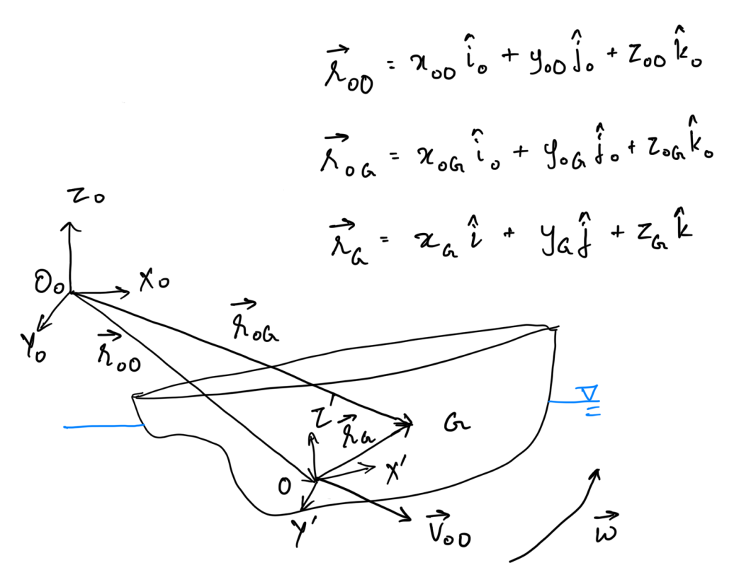
Consider a rigid body that is both translating and rotating as shown in Figure 5.1, whose center of gravity is denoted by \(G\) and the BCS origin is denoted by \(O\). The GCS frame is depicted as \(X_0Y_0Z_0\) with origin at \(O_0\) and the BCS frame is depicted as \(X'Y'Z'\) with origin \(O\). The three unit vectors along GCS are denoted as \((\hat{i}_0, \hat{j}_0, \hat{k}_0)\) and the corresponding unit vectors along BCS are denoted as \((\hat{i}, \hat{j}, \hat{k})\). The position vector from GCS origin to BCS origin expressed in GCS is denoted as shown in \(\eqref{eq-bcs-origin-vec-gcs}\). The position vector from GCS origin to center of gravity \(G\) expressed in GCS is denoted as shown in \(\eqref{eq-cog-vec-gcs}\). Let vector from BCS origin to the center of gravity \(G\) expressed in BCS be denoted as shown in \(\eqref{eq-cog-vec-bcs}\).

\[\begin{align} \vec{r}_{0O} = x_{0O} \hat{i}_0 + x_{0O} \hat{j}_0 + z_{0O} \hat{k}_0 \label{eq-bcs-origin-vec-gcs} \end{align}\]

\[\begin{align} \vec{r}_{0G} = x_{0G} \hat{i}_0 + x_{0G} \hat{j}_0 + z_{0G} \hat{k}_0 \label{eq-cog-vec-gcs} \end{align}\]

\[\begin{align} \vec{r}_G = x_G \hat{i} + y_G \hat{j} + z_G \hat{k} \label{eq-cog-vec-bcs} \end{align}\]

Let the velocity and acceleration of the center of gravity \(G\) expressed in GCS and BCS be denoted by \((\vec{v}_{0G}, \vec{a}_{0G})\) and \((\vec{v}_{G}, \vec{a}_{G})\) respectively. Similarly the angular velocity of the body expressed in GCS and BCS be denoted by \((\vec{\omega}_0, \vec{\alpha}_0)\) and \((\vec{\omega}, \vec{\alpha})\) respectively. Let the velocity and acceleration of the BCS origin \(O\) expressed in GCS and BCS be denoted by \((\vec{v}_{0O}, \vec{a}_{0O})\) and \((\vec{v}, \vec{a})\) respectively. Note that from the previous chapter, the vectors \(\vec{v}\) and \(\vec{\omega}\) are denoted as shown in \(\eqref{eq-vel-bcs}\) and \(\eqref{eq-ang-vel-bcs}\) respectively.

\[\begin{align} \vec{v} = u\hat{i} + v\hat{j} + w\hat{k} = \{\nu_1\} \label{eq-vel-bcs} \end{align}\]

\[\begin{align} \vec{\omega} = p\hat{i} + q\hat{j} + r\hat{k} = \{\nu_2\} \label{eq-ang-vel-bcs} \end{align}\]

It can be seen that the position vector \(\vec{r}_{0G}\) can be expressed as shown in \(\eqref{eq-position-vec-triangle-law}\) where \(\boldsymbol{R}\) is the rotation matrix.

\[\begin{align} \vec{r}_{0G} = \vec{r}_{0O} + \boldsymbol{R} \vec{r}_G \label{eq-position-vec-triangle-law} \end{align}\]

Differentiating \(\eqref{eq-position-vec-triangle-law}\) with respect to time yields \(\eqref{eq-vel-triangle-law}\).

\[\begin{align} \vec{v}_{0G} = \vec{v}_{0O} + \dot{\boldsymbol{R}} \vec{r}_G + \boldsymbol{R} \dot{\vec{r}}_G \label{eq-vel-triangle-law} \end{align}\]

Note that \(\dot{\vec{r}}_G = 0\) as in the BCS frame, the location of center of gravity \(G\) will not vary with time due to the rigid body assumption. The vector \(\vec{r}_G\) can be expressed from \(\eqref{eq-position-vec-triangle-law}\) as shown in \(\eqref{eq-rG-recast}\).

\[\begin{align} \vec{r}_G = \boldsymbol{R}^T (\vec{r}_{0G} - \vec{r}_{0O}) \label{eq-rG-recast} \end{align}\]

Substituting into \(\eqref{eq-vel-triangle-law}\) yields \(\eqref{eq-vel-triangle-law-1}\).

\[\begin{align} \vec{v}_{0G} = \vec{v}_{0O} + \dot{\boldsymbol{R}} \boldsymbol{R}^T (\vec{r}_{0G} - \vec{r}_{0O}) \label{eq-vel-triangle-law-1} \end{align}\]

The product \(\dot{\boldsymbol{R}} \boldsymbol{R}^T\) can be evaluated using symbolic python (sympy package) as seen in the code give below and the final expression in summarized in a compact form in \(\eqref{eq-RdotRT-compact-1}\). Note that \(s_1 = \sin(\phi)\), \(c_1 = \cos(\phi)\), \(s_2 = \sin(\theta)\), \(c_2=\cos(\theta)\), \(s_3 = \sin(\psi)\) and \(c_3 = \cos(\psi)\).

import sympy as sp

# Define symbols for angles and their time derivatives
phi, theta, psi = sp.symbols('phi theta psi', cls=sp.Function)
t = sp.symbols('t')
phi = phi(t)
theta = theta(t)
psi = psi(t)

# Define derivatives of angles with respect to time
phi_dot = sp.diff(phi, t)
theta_dot = sp.diff(theta, t)
psi_dot = sp.diff(psi, t)

# Define trigonometric functions
s1, c1 = sp.sin(phi), sp.cos(phi)
s2, c2 = sp.sin(theta), sp.cos(theta)
s3, c3 = sp.sin(psi), sp.cos(psi)

# Define the rotation matrix R
R = sp.Matrix([
    [c2*c3, -c1*s3 + s1*s2*c3, s1*s3 + c1*s2*c3],
    [c2*s3, c1*c3 + s1*s2*s3, -s1*c3 + c1*s2*s3],
    [-s2, s1*c2, c1*c2]
])

# Compute the time derivative of R
R_dot = R.diff(t)

# Compute R^T
R_T = R.transpose()

# Compute R_dot * R_T
result = R_dot * R_T

# Simplify the result
simplified_result = sp.simplify(result)
simplified_result

\[\begin{align} \dot{\boldsymbol{R}} \boldsymbol{R}^T = \begin{bmatrix} 0 & s_2\dot{\phi} - \dot{\psi} & s_3c_2\dot{\phi} + c_3\dot{\theta} \\ -s_2\dot{\phi} + \dot{\psi} & 0 & s_3\dot{\theta} - c_3c_2\dot{\phi} \\ -s_3c_2\dot{\phi} - c_3\dot{\theta} & -s_3\dot{\theta} + c_3c_2\dot{\phi} & 0 \end{bmatrix} \label{eq-RdotRT-compact-1} \end{align}\]

From the previous chapter it is seen that the angular velocity of the body \(\vec{\omega}\) is related to the Euler rates by \(\eqref{eq-ang-vel-bcs-repeat}\).

\[\begin{align} \vec{\omega} = \begin{bmatrix} \dot{\phi} - s_2 \dot{\psi} \\ c_1 \dot{\theta} + s_1c_2 \dot{\psi} \\ -s_1 \dot{\theta} + c_1c_2 \dot{\psi} \end{bmatrix} \label{eq-ang-vel-bcs-repeat} \end{align}\]

The angular velocity of the body expressed in GCS will be given by \(\eqref{eq-ang-vel-gcs}\). Note that the following code has been used to evaluate the final expression shown in \(\eqref{eq-ang-vel-gcs}\).

import sympy as sp

# Define symbols for angles and their time derivatives
phi, theta, psi = sp.symbols('phi theta psi', cls=sp.Function)
t = sp.symbols('t')
phi = phi(t)
theta = theta(t)
psi = psi(t)

# Define derivatives of angles with respect to time
phi_dot = sp.diff(phi, t)
theta_dot = sp.diff(theta, t)
psi_dot = sp.diff(psi, t)

# Define trigonometric functions
s1, c1 = sp.sin(phi), sp.cos(phi)
s2, c2 = sp.sin(theta), sp.cos(theta)
s3, c3 = sp.sin(psi), sp.cos(psi)

# Define the rotation matrix R
R = sp.Matrix([
    [c2*c3, -c1*s3 + s1*s2*c3, s1*s3 + c1*s2*c3],
    [c2*s3, c1*c3 + s1*s2*s3, -s1*c3 + c1*s2*s3],
    [-s2, s1*c2, c1*c2]
])

# Define angular velocity omega in BCS
omega = sp.Matrix([[phi_dot - s2*psi_dot], 
            [c1*theta_dot + s1*c2*psi_dot], 
            [-s1*theta_dot + c1*c2*psi_dot]])

# Angular velocity in GCS omega_0
omega_0 = R * omega

# Simplify the result
simplified_result = sp.simplify(omega_0)
simplified_result

\[\begin{align} \vec{\omega}_0 = \boldsymbol{R} \vec{\omega} = \begin{bmatrix} -s_3 \dot{\theta} + c_2c_3\dot{\phi} \\ s_3c_2\dot{\phi} + c_3 \dot{\theta} \\ - s_2 \dot{\phi} + \dot{\psi} \end{bmatrix} \label{eq-ang-vel-gcs} \end{align}\]

Expressing cross product as a matrix multiplication

Consider two vectors \(\vec{a} = a_1 \hat{i} + a_2 \hat{j} + a_3 \hat{k}\) and \(\vec{b} = b_1 \hat{i} + b_2 \hat{j} + b_3 \hat{k}\). The cross product \(\vec{a} \times \vec{b}\) is given by

\[\begin{align} \vec{a} \times \vec{b} = \begin{vmatrix} \hat{i} & \hat{j} & \hat{k} \\ a_1 & a_2 & a_3 \\ b_1 & b_2 & b_3 \end{vmatrix} = (a_2b_3 - a_3b_2) \hat{i} + (a_3b_1 - a_1b_3) \hat{j} + (a_1b_2 - a_2b_1) \hat{k} \end{align}\]

A skew symmetric matrix constructed from a vector is defined as

\[\begin{align} \boldsymbol{S}(\vec{a}) = \begin{bmatrix} 0 & -a_3 & a_2 \\ a_3 & 0 & -a_1 \\ -a_2 & a_1 & 0 \end{bmatrix} \end{align}\]

It can then be seen that the cross product \(\vec{a} \times \vec{b}\) can be expressed as

\[\begin{align} \vec{a} \times \vec{b} = \begin{bmatrix} a_2b_3 - a_3b_2 \\ a_3b_1 - a_1b_3 \\ a_1b_2 - a_2b_1 \end{bmatrix} = \begin{bmatrix} 0 & -a_3 & a_2 \\ a_3 & 0 & -a_1 \\ -a_2 & a_1 & 0 \end{bmatrix} \begin{bmatrix} b_1\\ b_2\\ b_3 \end{bmatrix} = \boldsymbol{S}(\vec{a}) \vec{b} \end{align}\]

Similarly,

\[\begin{align} \vec{a} \times \vec{b} = \begin{bmatrix} a_2b_3 - a_3b_2 \\ a_3b_1 - a_1b_3 \\ a_1b_2 - a_2b_1 \end{bmatrix} = \begin{bmatrix} 0 & b_3 & -b_2 \\ -b_3 & 0 & b_1 \\ b_2 & -b_1 & 0 \end{bmatrix} \begin{bmatrix} a_1\\ a_2\\ a_3 \end{bmatrix} = -\boldsymbol{S}(\vec{b})\vec{a} \end{align}\]

It can be seen that the right hand side of \(\eqref{eq-RdotRT-compact-1}\) is a skew symmetric matrix constructed from \(\vec{\omega}_0\) shown in \(\eqref{eq-ang-vel-gcs}\). Using the property of expressing cross product as a matrix multiplication, \(\eqref{eq-vel-triangle-law-1}\) can be written as shown in \(\eqref{eq-vel-triangle-law-2}\).

\[\begin{align} \vec{v}_{0G} = \vec{v}_{0O} + \vec{\omega}_0 \times (\vec{r}_{0G} - \vec{r}_{0O}) \label{eq-vel-triangle-law-2} \end{align}\]

Differentiating \(\eqref{eq-vel-triangle-law-2}\) with respect to time again yields \(\eqref{eq-acc-triangle-law-1}\).

\[\begin{align} \vec{a}_{0G} = \vec{a}_{0O} + \vec{\alpha}_0 \times (\vec{r}_{0G} - \vec{r}_{0O}) + \vec{\omega}_0 \times (\vec{v}_{0G} - \vec{v}_{0O}) \label{eq-acc-triangle-law-1} \end{align}\]

Substituting \((\vec{v}_{0G} - \vec{v}_{0O})\) from \(\eqref{eq-vel-triangle-law-2}\) into \(\eqref{eq-acc-triangle-law-1}\) yields \(\eqref{eq-acc-triangle-law-2}\).

\[\begin{align} \vec{a}_{0G} = \vec{a}_{0O} + \vec{\alpha}_0 \times (\vec{r}_{0G} - \vec{r}_{0O}) + \vec{\omega}_0 \times (\vec{\omega}_0 \times (\vec{r}_{0G} - \vec{r}_{0O})) \label{eq-acc-triangle-law-2} \end{align}\]

Newton’s second law for a point mass can be written as \(\eqref{eq-newtons-2nd-law}\) where \(\vec{F}_{0}\) is the force acting on the body expressed in GCS. \(m\) denotes the mass of the rigid body.

\[\begin{align} m \vec{a}_{0G} = \vec{F}_{0} \label{eq-newtons-2nd-law} \end{align}\]

Sustituting the acceleration of \(G\) expressed in GCS from \(\eqref{eq-acc-triangle-law-2}\) leads to \(\eqref{eq-newtons-eom}\).

\[\begin{align} m \left[\vec{a}_{0O} + \vec{\alpha}_0 \times (\vec{r}_{0G} - \vec{r}_{0O}) + \vec{\omega}_0 \times (\vec{\omega}_0 \times (\vec{r}_{0G} - \vec{r}_{0O}))\right] = \vec{F}_{0} \label{eq-newtons-eom} \end{align}\]

Notice that all the quantities in \(\eqref{eq-newtons-eom}\) are expressed in GCS frame. Premultiplying \(\boldsymbol{R}^T\) on both sides of \(\eqref{eq-newtons-eom}\) leads to translational equations of motion expressed in BCS frame as shown in \(\eqref{eq-newtons-eom-1}\).

\[\begin{align} m \left[\vec{a} + \vec{\alpha} \times \vec{r}_{G} + \vec{\omega} \times (\vec{\omega} \times \vec{r}_{G})\right] = \vec{F} \label{eq-newtons-eom-1} \end{align}\]

Note that \(\boldsymbol{R}^T(\vec{\alpha}_0 \times (\vec{r}_{0G} - \vec{r}_{0O})) = \vec{\alpha} \times \vec{r}_{G}\) and \(\boldsymbol{R}^T(\vec{\omega}_0 \times (\vec{\omega}_0 \times (\vec{r}_{0G} - \vec{r}_{0O}))) = \vec{\omega} \times (\vec{\omega} \times \vec{r}_{G})\). Transforming vectors to BCS and taking a cross product is equivalent to taking a cross product of vectors in GCS and transforming the resultant vector to BCS. \(\vec{F} = X \hat{i} + Y \hat{j} + Z \hat{k}\) in \(\eqref{eq-newtons-eom-1}\) represents the force acting of the rigid body expressed in BCS frame.

In BCS \(\vec{a} \neq \dot{\vec{v}}\) as BCS is a non-inertial frame of reference. Differentiation of velocity will yield acceleration only in an inertial frame. Instead \(\vec{a}\) can be expressed in terms of \(\dot{\vec{v}}\) and \(\vec{v}\) as shown in \(\eqref{eq-acc-vel-der-bcs}\).

\[\begin{align} \vec{a} = \boldsymbol{R}^T\vec{a}_{0O} = \boldsymbol{R}^T \frac{d}{dt} \vec{v}_{0O} = \boldsymbol{R}^T \frac{d}{dt} \left(\boldsymbol{R} \vec{v}\right) = \boldsymbol{R}^T\dot{\boldsymbol{R}}\vec{v} + \dot{\vec{v}} = \dot{\vec{v}} + \vec{\omega} \times \vec{v} \label{eq-acc-vel-der-bcs} \end{align}\]

Substituting \(\eqref{eq-acc-vel-der-bcs}\) into \(\eqref{eq-newtons-eom-1}\) results in the translational equations of motion in the vector form and are shown in \(\eqref{eq-newtons-eom-2}\).

\[\begin{align} m \left[\dot{\vec{v}} + \vec{\omega} \times \vec{v} + \vec{\alpha} \times \vec{r}_{G} + \vec{\omega} \times (\vec{\omega} \times \vec{r}_{G})\right] = \vec{F} \label{eq-newtons-eom-2} \end{align}\]

5.3 Rotational Equations of Motion

Let the angular momentum of the vessel about the center of gravity \(G\) expressed in GCS be denoted by \(\vec{L}_{0G}\). Let the angular momentum of the vessel about the center of gravity \(G\) expressed in BCS be denoted by \(\vec{L}_G\). Let the external moment on the vessel about the center of gravity \(G\) expressed in GCS be denoted by \(\vec{M}_{0G}\). The conservation of angular momentum for the vessel is shown by \(\eqref{eq-ang-momentum-conservation}\).

\[\begin{align} \frac{d}{dt} \vec{L}_{0G} = \vec{M}_{0G} \label{eq-ang-momentum-conservation} \end{align}\]

This can be recast as shown in \(\eqref{eq-ang-momentum-conservation-1}\).

\[\begin{align} \vec{M}_{0G} &= \frac{d}{dt} (\boldsymbol{R} \vec{L}_G) = \boldsymbol{R} \dot{\vec{L}}_G + \dot{\boldsymbol{R}} \vec{L}_G \nonumber \\ &= \boldsymbol{R} \left(\dot{\vec{L}}_G + \boldsymbol{R}^T \dot{\boldsymbol{R}} \vec{L}_{G} \right) \nonumber \\ &= \boldsymbol{R} \left(\dot{\vec{L}}_G + \vec{\omega} \times \vec{L}_{G} \right) \label{eq-ang-momentum-conservation-1} \end{align}\]

Rearranging yields \(\eqref{eq-ang-momentum-conservation-2}\).

\[\begin{align} \dot{\vec{L}}_G + \vec{\omega} \times \vec{L}_{G} = \boldsymbol{R}^T \vec{M}_{0G} \label{eq-ang-momentum-conservation-2} \end{align}\]

It is well known from rigid body mechanics that the angular momentum of the body in BCS \(\vec{L}_{G}\) can be expressed as the product of inertia tensor and the angular velocity as shown in \(\eqref{eq-ang-mom-inertia}\).

\[\begin{align} \vec{L}_{G} = \boldsymbol{I}_G \vec{\omega} \label{eq-ang-mom-inertia} \end{align}\]

The inertia tensor \(\boldsymbol{I}_G\) is defined as

\[\begin{align} \boldsymbol{I}_G = \begin{bmatrix} I_x^G & -I_{xy}^G & -I_{xz}^G \\ -I_{yx}^G & I_y^G & -I_{yz}^G \\ -I_{zx}^G & -I_{zy}^G & I_z^G \end{bmatrix} \end{align}\]

\(I_x^G\), \(I_y^G\) and \(I_z^G\) are the second mass moments of inertia. \(I_{xy}^G\), \(I_{xz}^G\), \(I_{yz}^G\), \(I_{yx}^G\), \(I_{zx}^G\) and \(I_{zy}^G\) are cross mass moments of inertia. The terms in the inertia tensor \(\boldsymbol{I}_G\) are defined with respect to a coordinate system that is parallel to the BCS but with its origin at the center of gravity \(G\).

The second mass moment of inertia \(I_x^G\) is defined as shown in \(\eqref{eq-IxG}\) where \(\mu\) represents the mass density of the body and the volume integral is performed over the volume \(V\) of the rigid body. Note that \((x - x_G)\), \((y - y_G)\) and \((z - z_G)\) represent the distance between the elemental volume \(dV\) and the center of gravity of the rigid body along directions parallel to the y and z axes of the BCS respectively. \(I_y^G\) and \(I_z^G\) are also defined in a similar manner.

\[\begin{align} I_x^G = I_{yy}^G + I_{zz}^G = \iiint_V \mu \left[(y - y_G)^2 + (z - z_G)^2\right] dV \label{eq-IxG} \end{align}\]

The cross mass moment of inertia \(I_{xy}^G\) is defined as shown in \(\eqref{eq-IxyG}\). The other terms \(I_{xz}^G\), \(I_{yz}^G\), \(I_{yx}^G\), \(I_{zx}^G\) and \(I_{zy}^G\) are defined in a similar manner.

\[\begin{align} I_{xy}^G = \iiint_V \mu (x - x_G) (y - y_G) dV \label{eq-IxyG} \end{align}\]

Note that for a rigid body \(\boldsymbol{I}_G\) is time invariant. The advantage of formulating the equations of motion in BCS is that the mass properties of the body are time invariant. On the other hand, when the equations of motion are formulated in GCS, the inertia tensor would be a time varying quantity.

Substituting \(\eqref{eq-ang-mom-inertia}\) into \(\eqref{eq-ang-momentum-conservation-2}\) results in \(\eqref{eq-rotational-eqn-cog}\).

\[\begin{align} \boldsymbol{I}_G \dot{\vec{\omega}} + \vec{\omega} \times \boldsymbol{I}_G \vec{\omega} = \boldsymbol{R}^T \vec{M}_{0G} \label{eq-rotational-eqn-cog} \end{align}\]

Let \(\vec{M} = K \hat{i} + M \hat{j} + N \hat{k}\) denote the external moment acting on the vessel about BCS origin \(O\) expressed in BCS. \(\vec{M}\) and \(\vec{M}_{0G}\) are related as shown in \(\eqref{eq-ext-moment}\) where \(\vec{F}\) is the external force acting on the body expressed in BCS.

\[\begin{align} \boldsymbol{R}^T \vec{M}_{0G} = \vec{M} - \vec{r}_G \times \vec{F} \label{eq-ext-moment} \end{align}\]

Substituting \(\eqref{eq-ext-moment}\) into \(\eqref{eq-rotational-eqn-cog}\) yields \(\eqref{eq-rotational-eqn-cog-1}\).

\[\begin{align} \boldsymbol{I}_G \dot{\vec{\omega}} + \vec{\omega} \times \boldsymbol{I}_G \vec{\omega} = \vec{M} - \vec{r}_G \times \vec{F} \label{eq-rotational-eqn-cog-1} \end{align}\]

Now \(\vec{F}\) can be substituted from \(\eqref{eq-newtons-eom-2}\) to yield \(\eqref{eq-euler-eom-1}\)

\[\begin{align} \boldsymbol{I}_G \dot{\vec{\omega}} &+ \vec{\omega} \times \boldsymbol{I}_G \vec{\omega} \nonumber \\ &= \vec{M} - \vec{r}_G \times m\left[\dot{\vec{v}} + \vec{\omega} \times \vec{v} + \vec{\alpha} \times \vec{r}_{G} + \vec{\omega} \times (\vec{\omega} \times \vec{r}_{G})\right] \label{eq-euler-eom-1} \end{align}\]

Rearranging yeilds \(\eqref{eq-euler-eom-2}\).

\[\begin{align} \boldsymbol{I}_G \dot{\vec{\omega}} &+ m \vec{r}_G \times (\dot{\vec{\omega}} \times \vec{r}_{G}) + \vec{\omega} \times \boldsymbol{I}_G \vec{\omega} \nonumber \\ &+ m \vec{r}_G \times (\vec{\omega} \times (\vec{\omega} \times \vec{r}_{G})) + m \vec{r}_G \times (\dot{\vec{v}} + \vec{\omega} \times \vec{v}) = \vec{M} \label{eq-euler-eom-2} \end{align}\]

Some of the terms can be simplified. Taking the first two terms together and applying the properties of vector cross product and expressing cross products as matrix multiplications yeilds \(\eqref{eq-inertia-simplify-1}\) and \(\eqref{eq-inertia-simplify-1a}\) respectively.

\[\begin{align} \boldsymbol{I}_G \dot{\vec{\omega}} + m \vec{r}_G \times (\dot{\vec{\omega}} \times \vec{r}_{G}) = \boldsymbol{I}_G \dot{\vec{\omega}} - m \vec{r}_G \times (\vec{r}_{G} \times \dot{\vec{\omega}}) \label{eq-inertia-simplify-1} \end{align}\]

\[\begin{align} \boldsymbol{I}_G \dot{\vec{\omega}} - m \vec{r}_G \times (\vec{r}_{G} \times \dot{\vec{\omega}}) = (\boldsymbol{I}_G - m \boldsymbol{S}(\vec{r}_G) \boldsymbol{S}(\vec{r}_G)) \dot{\vec{\omega}} = \boldsymbol{I}_O \dot{\vec{\omega}} \label{eq-inertia-simplify-1a} \end{align}\]

Note that \(\boldsymbol{I}_O\) in the last step is the inertia tensor defined with respect to BCS and is related to \(\boldsymbol{I}_G\) through the parallel axes theorem shown in \(\eqref{eq-parallel-axes-theorem}\).

\[\begin{align} \boldsymbol{I}_O = \boldsymbol{I}_G - m \boldsymbol{S}(\vec{r}_G) \boldsymbol{S}(\vec{r}_G) \label{eq-parallel-axes-theorem} \end{align}\]

Similarly, the third and fourth terms of \(\eqref{eq-euler-eom-2}\) can also be simplified using the Jacobi identity for triple cross products as shown in \(\eqref{eq-inertia-simplify-2}\), \(\eqref{eq-inertia-simplify-3}\) and \(\eqref{eq-inertia-simplify-4}\).

\[\begin{align} \vec{\omega} \times \boldsymbol{I}_G \vec{\omega} + m \vec{r}_G \times (\vec{\omega} \times (\vec{\omega} \times \vec{r}_{G})) = \vec{\omega} \times \boldsymbol{I}_G \vec{\omega} + m \vec{\omega} \times (\vec{r}_G \times (\vec{\omega} \times \vec{r}_{G})) \label{eq-inertia-simplify-2} \end{align}\]

\[\begin{align} \vec{\omega} \times \boldsymbol{I}_G \vec{\omega} + m \vec{\omega} \times (\vec{r}_G \times (\vec{\omega} \times \vec{r}_{G})) = \vec{\omega} \times \boldsymbol{I}_G \vec{\omega} - m \vec{\omega} \times (\vec{r}_G \times (\vec{r}_{G} \times \vec{\omega})) \label{eq-inertia-simplify-3} \end{align}\]

\[\begin{align} \vec{\omega} \times \boldsymbol{I}_G \vec{\omega} - m \vec{\omega} \times (\vec{r}_G \times (\vec{r}_{G} \times \vec{\omega})) = \vec{\omega} \times (\boldsymbol{I}_G - m \boldsymbol{S}(\vec{r}_G) \boldsymbol{S}(\vec{r}_G)) \vec{\omega} = \vec{\omega} \times \boldsymbol{I}_O \vec{\omega} \label{eq-inertia-simplify-4} \end{align}\]

Substituting final expressions from \(\eqref{eq-inertia-simplify-1a}\) and \(\eqref{eq-inertia-simplify-4}\) into \(\eqref{eq-euler-eom-2}\) yeilds the rotational equations in the vector form as shown in \(\eqref{eq-euler-eom-3}\).

\[\begin{align} \boldsymbol{I}_O \dot{\vec{\omega}} + \vec{\omega} \times \boldsymbol{I}_O \vec{\omega} + m \vec{r}_G \times (\dot{\vec{v}} + \vec{\omega} \times \vec{v}) = \vec{M} \label{eq-euler-eom-3} \end{align}\]

5.4 Complete Equations of Motion for a Rigid Body

The equations of motion governing the dynamics of a rigid body are given by \(\eqref{eq-newtons-eom-final}\) and \(\eqref{eq-euler-eom-final}\).

\[\begin{align} m \left[\dot{\vec{v}} + \vec{\omega} \times \vec{v} + \vec{\alpha} \times \vec{r}_{G} + \vec{\omega} \times (\vec{\omega} \times \vec{r}_{G})\right] = \vec{F} \label{eq-newtons-eom-final} \end{align}\]

\[\begin{align} \boldsymbol{I}_O \dot{\vec{\omega}} + \vec{\omega} \times \boldsymbol{I}_O \vec{\omega} + m \vec{r}_G \times (\dot{\vec{v}} + \vec{\omega} \times \vec{v}) = \vec{M} \label{eq-euler-eom-final} \end{align}\]

When expanded, these form six equations, with one corresponding to each degree of freedom and are shown in (\(\ref{eq-eom-expanded-1}\) - \(\ref{eq-eom-expanded-6}\)).

\[\begin{align} m\left[\dot{u} - vr + wq - x_G(q^2 + r^2) + y_G(pq - \dot{r}) + z_G (pr + \dot{q})\right] = X \label{eq-eom-expanded-1} \end{align}\]

\[\begin{align} m \left[\dot{v} - wp + ur - y_G (r^2 + p^2) + z_G (qr - \dot{p}) + x_G (qp + \dot{r})\right] = Y \label{eq-eom-expanded-2} \end{align}\]

\[\begin{align} m \left[\dot{w} - uq + vp - z_G(p^2 + q^2) + x_G (rp - \dot{q}) + y_G (rq + \dot{p})\right] = Z \label{eq-eom-expanded-3} \end{align}\]

\[\begin{align} I_x \dot{p} + (I_z - I_y) qr &- (\dot{r} + pq) I_{xz} + (r^2 - q^2) I_{yz} + (pr - \dot{q}) I_{xy} \nonumber \\ &+ m \left[y_G(\dot{w} - uq + vp) - z_G(\dot{v} -wp + ur)\right] = K \label{eq-eom-expanded-4} \end{align}\]

\[\begin{align} I_y \dot{q} + (I_x - I_z) rp &- (\dot{p} + qr) I_{yx} + (p^2 - r^2) I_{zx} + (qp - \dot{r}) I_{yz} \nonumber \\ &+ m \left[z_G (\dot{u} - vr + wq) - x_G (\dot{w} - uq + vp)\right] = M \label{eq-eom-expanded-5} \end{align}\]

\[\begin{align} I_z \dot{r} + (I_y - I_x) pq &- (\dot{q} + rp) I_{zy} + (q^2 - p^2) I_{xy} + (rq - \dot{p})I_{zx} \nonumber \\ &+ m \left[x_G(\dot{v} - wp + ur) - y_G(\dot{u} - vr + wq)\right] = N \label{eq-eom-expanded-6} \end{align}\]

These equations can be represented in a compact matrix form as shown in \(\eqref{eq-eom-matrix-form}\), where \(\boldsymbol{M}_{RB}\) is a \(6 \times 6\) rigid body mass matrix, \(\boldsymbol{C}_{RB}\left(\{\nu\}\right)\) is the \(6 \times 6\) velocity dependent Coriolis matrix and \(\{\tau_{RB}\}\) is the \(6 \times 1\) external force and moment vector.

\[\begin{align} \boldsymbol{M}_{RB} \{\dot{\nu}\} + \boldsymbol{C}_{RB}\left(\{\nu\}\right)\{\nu\} = \{\tau_{RB}\} \label{eq-eom-matrix-form} \end{align}\]

The rigid body mass matrix \(\boldsymbol{M}_{RB}\) is shown in \(\eqref{eq-mass-matrix}\), where \(\boldsymbol{I}_{3 \times 3}\) is a \(3 \times 3\) identity matrix.

\[\begin{align} \boldsymbol{M}_{RB} &= \begin{bmatrix} m\boldsymbol{I}_{3 \times 3} & -m \boldsymbol{S}(\vec{r}_G) \\ m \boldsymbol{S}(\vec{r}_G) & \boldsymbol{I}_O \end{bmatrix} \nonumber \\ &= \begin{bmatrix} m & 0 & 0 & 0 & mz_G & -my_G \\ 0 & m & 0 & -mz_G & 0 & mx_G\\ 0 & 0 & m & my_G & -mx_G & 0 \\ 0 & -mz_G & my_G & I_x^O & -I_{xy}^O & -I_{xz}^O \\ mz_G & 0 & -mx_G & -I_{yx}^O & I_y^O & -I_{yz}^O \\ -my_G & mx_G & 0 & -I_{zx}^O & -I_{zy}^O & I_z^O \end{bmatrix} \label{eq-mass-matrix} \end{align}\]

The Coriolis matrix can be parameterized in terms of the mass matrix as shown in \(\eqref{eq-coriolis-mass-param}\), where \(\boldsymbol{0}_{3 \times 3}\) is a \(3 \times 3\) matrix of zeros. Note that \(\boldsymbol{M}_{11} = m\boldsymbol{I}_{3 \times 3}\), \(\boldsymbol{M}_{12} = -\boldsymbol{M}_{21} = -m \boldsymbol{S}(\vec{r}_G)\) and \(\boldsymbol{M}_{22} = \boldsymbol{I}_O\).

\[\begin{align} \boldsymbol{C}_{RB} \left(\{\nu\}\right) = \begin{bmatrix} \boldsymbol{0}_{3 \times 3} & -\boldsymbol{S}\left(\boldsymbol{M}_{11}\{\nu_1\} + \boldsymbol{M}_{12}\{\nu_2\}\right) \\ -\boldsymbol{S}\left(\boldsymbol{M}_{11}\{\nu_1\} + \boldsymbol{M}_{12}\{\nu_2\}\right) & -\boldsymbol{S}\left(\boldsymbol{M}_{21}\{\nu_1\} + \boldsymbol{M}_{22}\{\nu_2\}\right) \end{bmatrix} \label{eq-coriolis-mass-param} \end{align}\]

Defining a state vector of size \(12 \times 1\) as shown in \(\eqref{eq-state}\), the kinematic and dynamic equations can be expressed together as shown in \(\eqref{eq-kinematics-dynamics}\).

\[\begin{align} \{x\} = \begin{bmatrix} u & v & w & p & q & r & x_{0O} & y_{0O} & z_{0O} & \phi & \theta & \psi \end{bmatrix}^T \label{eq-state} \end{align}\]

\[\begin{align} \{\dot{x}\} = \begin{bmatrix} \{\dot{\nu}\} \\ \{\dot{\eta}\} \end{bmatrix} = \begin{bmatrix} \boldsymbol{M}_{RB}^{-1} \left(\{\tau_{RB}\} - \boldsymbol{C}_{RB}\left(\{\nu\}\right)\{\nu\}\right) \\ \boldsymbol{J}(\{\eta_2\}) \{\nu\} \end{bmatrix} \label{eq-kinematics-dynamics} \end{align}\]

If the external forces and moments \(\{\tau_{RB}\}\) are known, then the velocities and pose of the body can be calculated by solving the matrix differential equation shown in \(\eqref{eq-kinematics-dynamics}\).

5.5 Linearized Equations of Motion for a Rigid Body

For a ship or an offshore floating platform, the external forces acting on the body are due to the surrounding fluid. In general these hydrodynamic and hydrostatic forces acting on the body are strongly coupled to the motion of the body. This makes it very difficult to analyze the motions of ships and offshore platforms. In order to make the problem tenable the equations of motion are linearized. The linearization is only valid when the motions are small. However, the linearization allows for the principle of superposition. Thus the forces and external moments can be separated into their respective components and the response of the structure can be obtained by calculating the response of the structure to these component forces and moments.

When the amplitude of motions is assumed to be small, the nonlinear terms that involve the product of two or more small quantities can be neglected. In this case the dynamic equations of motion reduce to \(\eqref{eq-eom-matrix-form-linear}\).

\[\begin{align} \boldsymbol{M}_{RB} \{\dot{\nu}\} = \{\tau_{RB}\} \label{eq-eom-matrix-form-linear} \end{align}\]

The linearized kinematic and dynamic equations can be expressed together as shown in \(\eqref{eq-kinematics-dynamics-linear}\).

\[\begin{align} \{\dot{x}\} = \begin{bmatrix} \{\dot{\nu}\} \\ \{\dot{\eta}\} \end{bmatrix} = \begin{bmatrix} \boldsymbol{M}_{RB}^{-1} \{\tau_{RB}\} \\ \{\nu\} \end{bmatrix} \label{eq-kinematics-dynamics-linear} \end{align}\]

The next chapters will rely on the principle of superposition and separate the the total force and moment acting on the body into its components.

5.6 Exercises

Throughout, the BCS is the body frame of Chapter 4 — \(x\) along the bow, \(y\) to port, \(z\) up — with its origin \(O\) at midship, on the centreline, at the loaded waterline. All six equations are written about \(O\), not about \(G\), exactly as in \(\eqref{eq-eom-expanded-1}\)–\(\eqref{eq-eom-expanded-6}\). Use \(g = 9.81\) m/s\(^2\) and \(\rho = 1025\) kg/m\(^3\).

Every problem can be solved with the results of this chapter — the Newton–Euler equations \(\eqref{eq-newtons-eom-final}\) and \(\eqref{eq-euler-eom-final}\), their expanded scalar forms, the mass matrix \(\eqref{eq-mass-matrix}\), the Coriolis parameterization \(\eqref{eq-coriolis-mass-param}\), the parallel axes theorem \(\eqref{eq-parallel-axes-theorem}\), the moment transfer relation \(\eqref{eq-ext-moment}\) and the combined model \(\eqref{eq-kinematics-dynamics}\) — together with the kinematics of Chapter 4. No hydrodynamics is required anywhere: added mass, damping and wave loads are not part of this chapter, and wherever a force or moment acts on the vessel its value is given to you. Where a hydrostatic restoring moment is needed it is supplied as \(\rho g \nabla\, GM\), which you already know.

Several problems ask you to derive a result before using it numerically; the derivation carries most of the marks. The vessel dimensions are representative of a real ship and serve only to give the numbers a realistic scale.

The vessel and the two points these problems refer to

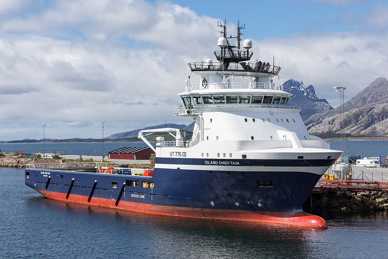
Most of the problems below concern one ship: a platform supply vessel of the kind shown in Figure 5.2, of length \(85\) m, beam \(20\) m and loaded draft \(6.5\) m. It is a useful test case because it is small enough to have a substantial \(\vec{r}_G\) relative to its size, so the coupling terms in \(\eqref{eq-mass-matrix}\) — which vanish only if the origin is placed at \(G\) — are large enough to matter.

Figure 5.2: A platform supply vessel. The open working deck aft, the accommodation forward and the deep skeg give a hull whose centre of gravity is neither at midship nor at the waterline, which is exactly the situation the mass matrix \(\eqref{eq-mass-matrix}\) is written for. Photo: JoachimKohler-HB, CC BY-SA 4.0, via Wikimedia Commons.

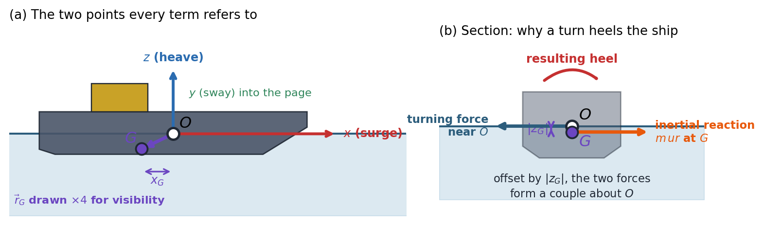
Every term in this chapter’s equations refers to one of two points: the BCS origin \(O\), which is bolted to the hull, and the centre of gravity \(G\), which moves whenever cargo, fuel or ballast moves. Figure 5.3 shows both, together with the geometry behind Problem 3.

Figure 5.3: (a) The BCS origin \(O\) and the centre of gravity \(G\) on the supply vessel, with the offset \(\vec{r}_G\) between them drawn four times its true size so that it can be seen at all. Surge, sway and heave are translations along the body axes; roll, pitch and yaw are rotations about them. (b) The geometry behind Problem 3: the force that turns the ship acts near the waterline while the inertia of the ship reacts at \(G\), and because the two are offset vertically by \(|z_G|\) they form a couple that heels the vessel.

1. The mass matrix of a supply vessel. The vessel of Figure 5.2 has mass \(m = 6.0\times10^{6}\) kg. Its centre of gravity lies at \(\vec{r}_G = [-2.5,\ 0,\ -1.2]^T\) m in the BCS — a little aft of midship and a little below the waterline. Its radii of gyration about \(G\) are \(k_x = 7.2\) m, \(k_y = 21.0\) m and \(k_z = 21.5\) m, and the hull is port–starboard symmetric so that \(I_{xy}^G = I_{yz}^G = 0\), while \(I_{xz}^G = 2.5\times10^{7}\) kg·m\(^2\).

   1. Write down \(\boldsymbol{I}_G\). Then expand \(-m\boldsymbol{S}(\vec{r}_G)\boldsymbol{S}(\vec{r}_G)\) in \(\eqref{eq-parallel-axes-theorem}\) using the identity \(\boldsymbol{S}(\vec{a})\boldsymbol{S}(\vec{a}) = \vec{a}\vec{a}^T - (\vec{a}\cdot\vec{a})\boldsymbol{I}\), and hence show that the diagonal entries reproduce the familiar scalar results \(I_x^O = I_x^G + m(y_G^2 + z_G^2)\) and so on, while the off-diagonal entry gives \(I_{xz}^O = I_{xz}^G + m x_G z_G\). Evaluate \(\boldsymbol{I}_O\).
   2. Assemble \(\boldsymbol{M}_{RB}\) from \(\eqref{eq-mass-matrix}\) and confirm that it is symmetric. Which property of \(\boldsymbol{S}\) makes the two off-diagonal blocks transposes of one another?
   3. The kinetic energy of the body is \(T = \tfrac{1}{2}\{\nu\}^T\boldsymbol{M}_{RB}\{\nu\}\). Use this to argue that \(\boldsymbol{M}_{RB}\) must be positive definite, and verify it numerically from its eigenvalues. What would a zero eigenvalue mean physically?
   4. Rebuild the matrix with the origin moved to \(G\). Show that both off-diagonal blocks vanish. List the pairs of degrees of freedom that the original off-diagonal terms coupled, and give the size of the largest coupling as a fraction of \(\sqrt{M_{ii}M_{jj}}\) for that pair.
   5. The matrix is plainly simpler at \(G\). Give the reason, already met in Chapter 4, why the equations are nevertheless written about a fixed geometric point.

2. What an accelerometer on the bridge actually measures. A motion sensor is bolted to the bridge of the vessel of Problem 1 at \(\vec{r}_P = [28,\ 0,\ 16]^T\) m in the BCS. At one instant the vessel has \[\{\nu_1\} = [5.00,\ 0.30,\ -0.20]^T \text{ m/s}, \qquad \{\nu_2\} = [0.080,\ 0.030,\ 0.020]^T \text{ rad/s}\] with rates \(\{\dot{v}_1\} = [0.10,\ -0.05,\ 0.40]^T\) m/s\(^2\) and \(\{\dot{v}_2\} = [0.050,\ -0.020,\ 0.010]^T\) rad/s\(^2\).

   1. Repeat the argument that led to \(\eqref{eq-newtons-eom-1}\), but for an arbitrary material point \(P\) of the body rather than for \(G\), to show that the acceleration of \(P\) expressed in the BCS is \[\vec{a}_P = \dot{\vec{v}} + \vec{\omega}\times\vec{v} + \vec{\alpha}\times\vec{r}_P + \vec{\omega}\times(\vec{\omega}\times\vec{r}_P)\] Identify which terms vanish if the vessel does not rotate, and which vanish if it rotates at a constant rate.
   2. Evaluate \(\vec{a}_P\) and the acceleration \(\vec{a}_O\) of the BCS origin. What fraction of the total does the rotational part contribute?
   3. The vertical channel of this sensor is often read directly as the heave acceleration. Compute the error committed by reading \((\vec{a}_P)_z\) as \(\dot{w}\), and identify which single term is responsible for most of it.
   4. Show that in a steady turn — constant \(u\) and \(r\), everything else zero — only two of the four terms survive. Evaluate the steady lateral acceleration felt on the bridge for \(u = 6.0\) m/s and \(r = 0.050\) rad/s, and express it as a fraction of \(g\).
   5. Where along the hull should the sensor be mounted so that its vertical channel is least contaminated by rotation? Is such a location practical, and what do designers do instead?

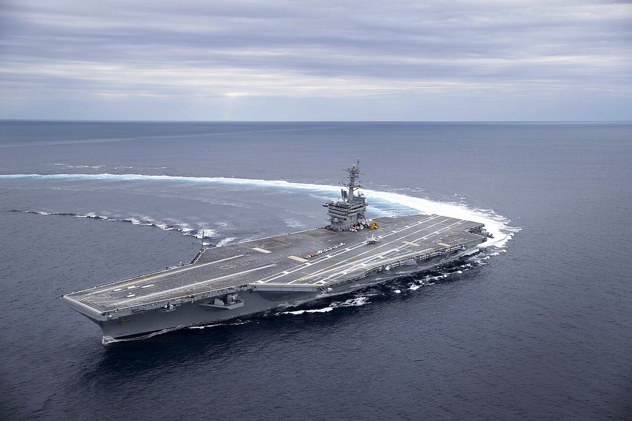
Figure 5.4 shows what this problem is about. The curved wake records the turn; the flight deck, which should be horizontal, is visibly tilted. No wave is doing that — the ship is heeling because of its own inertia, and the roll equation \(\eqref{eq-eom-expanded-4}\) is enough to say by how much.

Figure 5.4: An aircraft carrier during a high-speed turn on sea trials. The wake shows the turning circle and the deck shows the heel that goes with it. Photo: U.S. Navy, public domain, via Wikimedia Commons.

3. Why a ship heels in a turn. The vessel of Problem 1 is in a steady turn to port: \(u = 6.0\) m/s, \(v = -0.40\) m/s, \(w = 0\), \(p = q = 0\) and \(r = 0.050\) rad/s, every one of them constant. Take \(GM = 1.8\) m.

   1. Impose these conditions on the roll equation \(\eqref{eq-eom-expanded-4}\) and show that it reduces to \(K = r^2 I_{yz} - m z_G u r\), and hence, for a port–starboard symmetric hull, to \(K = -m z_G u r\). Explain in words what each surviving factor represents.
   2. Evaluate \(K\) for this vessel.
   3. In a steady heel the only other roll moment is the hydrostatic righting moment, which for small angles is \(-\rho g \nabla\, GM\, \phi\) with \(\rho\nabla = m\). Equate the two and find the heel angle \(\phi\). Does the vessel lean into the turn or out of it?
   4. The vessel is re-ballasted for a deck cargo so that \(G\) rises to \(z_G = +0.8\) m, above the waterline, with \(GM\) unchanged. Recompute \(\phi\) and explain the reversal in one sentence.
   5. Real ships in a hard turn usually heel outwards, whichever side \(G\) lies. Identify the assumption in this problem that is responsible for the discrepancy, and state what would have to be known to get the sign right in general.

4. The Coriolis matrix can do no work. This problem establishes a property of \(\eqref{eq-eom-matrix-form}\) that every simulation of it should be tested against.

   1. Using only \(\boldsymbol{S}^T = -\boldsymbol{S}\), show from the parameterization \(\eqref{eq-coriolis-mass-param}\) that \(\boldsymbol{C}_{RB}^T = -\boldsymbol{C}_{RB}\), whatever the velocity.
   2. Hence show that \(\{\nu\}^T\boldsymbol{C}_{RB}(\{\nu\})\{\nu\} = 0\) for every \(\{\nu\}\), and verify numerically for the state of Problem 2.
   3. Differentiate the kinetic energy \(T = \tfrac{1}{2}\{\nu\}^T\boldsymbol{M}_{RB}\{\nu\}\) and use \(\eqref{eq-eom-matrix-form}\) together with part (b) to prove that \(\dot{T} = \{\nu\}^T\{\tau_{RB}\}\). State in one sentence what this says physically.
   4. For the vessel of Problem 1 in the state of Problem 2, with \[\{\tau_{RB}\} = [3.0\times10^{5},\ -8.0\times10^{4},\ 2.0\times10^{5},\ 5.0\times10^{5},\ -1.2\times10^{6},\ 9.0\times10^{5}]^T\] in N and N·m, compute \(\dot{T}\) from the right-hand side, and independently from \(\{\nu\}^T\boldsymbol{M}_{RB}\{\dot{\nu}\}\) with \(\{\dot{\nu}\}\) obtained from \(\eqref{eq-eom-matrix-form}\). Confirm they agree.
   5. A student’s simulator builds \(\boldsymbol{C}_{RB}\) with the sign of its lower-left block flipped. Show that the matrix is then no longer skew-symmetric, and describe the single cheapest numerical test that would expose the error.

5. A steady turn is not an unaccelerated state. The vessel of Problem 1 holds the steady turn of Problem 3: \(u = 6.0\) m/s, \(v = -0.40\) m/s, \(w = 0\), \(p = q = 0\), \(r = 0.050\) rad/s, all constant.

   1. Write down \(\{\dot{\nu}\}\) for this motion, and say in one sentence why every entry is zero even though the vessel is going round in a circle.
   2. Substitute the state into the six expanded equations \(\eqref{eq-eom-expanded-1}\)–\(\eqref{eq-eom-expanded-6}\) and derive closed-form expressions for \(X\), \(Y\), \(Z\), \(K\), \(M\) and \(N\).
   3. Evaluate all six for this vessel.
   4. Two of the six have a simple interpretation: identify them and give it. Which one would be absent if the origin were at \(G\)?
   5. Resolve the apparent paradox in the title of this problem: how can the required forces be non-zero when every component of \(\{\dot{\nu}\}\) vanishes?

6. A pure surge force does not produce a pure surge acceleration. The vessel of Problem 1 lies at rest, \(\{\nu\} = \boldsymbol{0}\), when a towline along the body \(x\) axis through the origin suddenly comes taut with \(X = 5.0\times10^{5}\) N. No other force or moment acts.

   1. Show that \(\boldsymbol{C}_{RB}(\{\nu\})\{\nu\} = \boldsymbol{0}\) when \(\{\nu\} = \boldsymbol{0}\), so that \(\eqref{eq-eom-matrix-form}\) reduces to \(\{\dot{\nu}\} = \boldsymbol{M}_{RB}^{-1}\{\tau_{RB}\}\) at this instant.
   2. Compute \(\{\dot{\nu}\}\). Which components besides \(\dot{u}\) are non-zero?
   3. Identify the entries of \(\boldsymbol{M}_{RB}\) responsible, and explain the coupling in words — what is it about the geometry of this ship that makes a horizontal pull start a pitching motion?
   4. Find the pair \((X, M)\) that would produce a pure surge acceleration of the same magnitude as in (b), with every other component of \(\{\dot{\nu}\}\) exactly zero.
   5. If the origin were placed at \(G\), a force through \(G\) along \(x\) would produce pure surge acceleration. Does that mean the coupling in (b) is a mere artefact of a bad choice of origin? Answer carefully, distinguishing the line of action of the force from the choice of reference point.

7. The same physics from two different origins. A crane on the vessel of Problem 1 holds a load out over the port quarter. The load line applies a force \(\vec{F} = [0,\ -1.80\times10^{5},\ -9.00\times10^{5}]^T\) N at the point \(\vec{r}_A = [-18,\ 9,\ 12]^T\) m in the BCS. The vessel is momentarily at rest.

   1. Compute the moment of this force about \(O\) and about \(G\), and verify the relation \(\eqref{eq-ext-moment}\) numerically.
   2. Using the \(O\)-based mass matrix of Problem 1, assemble \(\{\tau_{RB}\}\) and solve for \(\{\dot{\nu}\}\).
   3. Now repeat the whole calculation with the BCS origin moved to \(G\): build the new mass matrix, express the same physical force and its moment about \(G\), and solve for the accelerations \(\{\dot{\nu}\}^G\).
   4. The two answers are numerically different. Show that they nevertheless describe the same motion, by checking that the angular accelerations are identical and that the linear accelerations satisfy \(\vec{a}_G = \vec{a}_O + \vec{\alpha}\times\vec{r}_G\). (Note that with the vessel at rest, \(\{\dot{\nu}\}\) is the acceleration.)
   5. In part (c) the linear acceleration comes out as exactly \(\vec{F}/m\). Explain why that had to happen, and say which of the two formulations you would prefer when writing a general purpose simulator.

8. A released subsea module tumbles. A rectangular subsea module of mass \(4.5\times10^{4}\) kg and outside dimensions \(6.0\) m (\(x\)) \(\times\ 3.0\) m (\(y\)) \(\times\ 2.0\) m (\(z\)), of uniform density, is released in mid-water. Place the BCS origin at \(G\) and, for this problem only, neglect every hydrodynamic force and moment, so that the net external force and moment on the module are zero.

   1. Compute the three principal moments of inertia and confirm that they are distinct.
   2. Show that \(\eqref{eq-euler-eom-final}\) reduces for this body to Euler’s equations \(I_x\dot{p} = (I_y - I_z)qr\), \(I_y\dot{q} = (I_z - I_x)rp\), \(I_z\dot{r} = (I_x - I_y)pq\), stating which terms drop out and why.
   3. Linearize about a steady spin of rate \(\Omega\) about each principal axis in turn. Show that two of the three give bounded oscillations and one gives exponential growth, and evaluate the oscillation frequencies and the growth rate for \(\Omega = 1.2\) rad/s.
   4. Integrate the equations numerically from \(\vec{\omega}(0) = [10^{-3},\ 1.2,\ 10^{-3}]^T\) rad/s over \(60\) s and report the times at which the spin about the intermediate axis reverses sign.
   5. About which axis should the module be spun if it must hold its attitude? Comment on what the neglected hydrodynamic moments would do to this picture.

9. Lifting a load changes the ship’s dynamics. The vessel of Problem 1 lifts a \(2.5\times10^{5}\) kg module and holds it fixed relative to the hull at \(\vec{r}_L = [-18,\ 9,\ 20]^T\) m in the BCS — on the port quarter and \(20\) m above the waterline. Treat the module as a point mass, and take the vessel’s own mass, centre of gravity and inertia tensor about its own centre of gravity to be unchanged.

   1. Compute the mass, the new centre of gravity \(\vec{r}_G'\) of the combined body, and comment on the direction in which \(G\) has moved.
   2. Using \(\eqref{eq-parallel-axes-theorem}\) on each part separately, compute the inertia tensor of the combined body about its new centre of gravity, and then about \(O\).
   3. Assemble the new \(\boldsymbol{M}_{RB}\) and state which entries are non-zero now that were zero before.
   4. Repeat the steady turn of Problem 3 for the loaded vessel, taking \(GM = 1.35\) m because of the added weight so high up. Compare the heel angle with the unloaded value.
   5. Which products of inertia have become non-zero, and which pairs of degrees of freedom do they couple? Name one practical consequence for the crane operator.

10. Programming Problem: A six degree of freedom simulation. The vessel of Problem 1 starts at rest with its pose \(\{\eta\} = \boldsymbol{0}\), i.e. at the GCS origin, upright and heading along \(X_0\). From \(t = 0\) a constant body-frame load \(\{\tau_{RB}\} = [2.0\times10^{5},\ 0,\ 0,\ 0,\ 0,\ 1.5\times10^{6}]^T\) in N and N·m is applied — a steady ahead thrust together with a steady turning moment.

    1. Write out the twelve first-order differential equations of \(\eqref{eq-kinematics-dynamics}\) that have to be integrated, naming the matrices that appear in each half.
    2. Integrate them for \(90\) s and report the full state at the end.
    3. Verify the energy identity of Problem 4 numerically, by comparing \(T(90) - T(0)\) with \(\int_0^{90}\{\nu\}^T\{\tau_{RB}\}\,\mathrm{d}t\).
    4. The vessel ends up rolling and pitching by several degrees and well below its starting draft, even though the applied load has no vertical or rolling component. Explain where those motions come from.
    5. The speed never settles to a steady value. Say why, and name the two classes of force that a realistic model would have to add before this simulation could be used to predict a turning circle.

Answer Key

Problem 1 — The mass matrix of a supply vessel

• (a) With \(\boldsymbol{S}(\vec{a})\boldsymbol{S}(\vec{a}) = \vec{a}\vec{a}^T - (\vec{a}\cdot\vec{a})\boldsymbol{I}\), \(-m\boldsymbol{S}(\vec{r}_G)\boldsymbol{S}(\vec{r}_G) = m\left[(\vec{r}_G\cdot\vec{r}_G)\boldsymbol{I} - \vec{r}_G\vec{r}_G^T\right]\). Its \((1,1)\) entry is \(m(x_G^2+y_G^2+z_G^2 - x_G^2) = m(y_G^2+z_G^2)\), which added to \(I_x^G\) is exactly the scalar parallel axes result; the same holds for the other two diagonals. Its \((1,3)\) entry is \(-m x_G z_G\), and since the tensor carries \(-I_{xz}\) in that slot, \(I_{xz}^O = I_{xz}^G + m x_G z_G\). Numerically \[\boldsymbol{I}_G = \begin{bmatrix} 3.110\!\times\!10^{8} & 0 & -2.500\!\times\!10^{7} \\ 0 & 2.646\!\times\!10^{9} & 0 \\ -2.500\!\times\!10^{7} & 0 & 2.774\!\times\!10^{9} \end{bmatrix}, \qquad \boldsymbol{I}_O = \begin{bmatrix} 3.197\!\times\!10^{8} & 0 & -4.300\!\times\!10^{7} \\ 0 & 2.692\!\times\!10^{9} & 0 \\ -4.300\!\times\!10^{7} & 0 & 2.811\!\times\!10^{9} \end{bmatrix}\] so \(I_x^O = 3.1968 \times 10^{8}\), \(I_y^O = 2.6921 \times 10^{9}\), \(I_z^O = 2.8110 \times 10^{9}\) kg·m\(^2\) and \(I_{xz}^O = 4.3000 \times 10^{7}\) kg·m\(^2\).
• (b) \[\boldsymbol{M}_{RB} = \begin{bmatrix} 6.000\!\times\!10^{6} & 0 & 0 & 0 & -7.200\!\times\!10^{6} & 0 \\ 0 & 6.000\!\times\!10^{6} & 0 & 7.200\!\times\!10^{6} & 0 & -1.500\!\times\!10^{7} \\ 0 & 0 & 6.000\!\times\!10^{6} & 0 & 1.500\!\times\!10^{7} & 0 \\ 0 & 7.200\!\times\!10^{6} & 0 & 3.197\!\times\!10^{8} & 0 & -4.300\!\times\!10^{7} \\ -7.200\!\times\!10^{6} & 0 & 1.500\!\times\!10^{7} & 0 & 2.692\!\times\!10^{9} & 0 \\ 0 & -1.500\!\times\!10^{7} & 0 & -4.300\!\times\!10^{7} & 0 & 2.811\!\times\!10^{9} \end{bmatrix}\] The largest asymmetry is \(0.0e+00\), i.e. exactly zero. Symmetry follows because \(\boldsymbol{I}_O\) is symmetric and because \(\boldsymbol{S}\) is skew: \((-m\boldsymbol{S}(\vec{r}_G))^T = +m\boldsymbol{S}(\vec{r}_G)\), which is precisely the lower-left block.
• (c) For any non-zero velocity the body has strictly positive kinetic energy, so \(\{\nu\}^T\boldsymbol{M}_{RB}\{\nu\} > 0\) for all \(\{\nu\} \neq 0\), which is the definition of positive definiteness. The eigenvalues are \(5.7647 \times 10^{6}\) to \(2.8118 \times 10^{9}\), all positive. A zero eigenvalue would mean some non-zero combination of surge, sway, heave, roll, pitch and yaw carried no kinetic energy at all — impossible for a body with mass, and in a simulation it would make \(\boldsymbol{M}_{RB}\) singular and the accelerations undefined.
• (d) With \(O\) at \(G\), \(\vec{r}_G = 0\) so \(\boldsymbol{S}(\vec{r}_G) = \boldsymbol{0}\) and the matrix collapses to \(\operatorname{diag}(m,m,m) \oplus \boldsymbol{I}_G\), block diagonal. The off-diagonal terms had coupled surge–pitch (\(\pm7.20 \times 10^{6}\)), sway–roll (\(\pm7.20 \times 10^{6}\)), sway–yaw (\(\pm1.50 \times 10^{7}\)), heave–pitch (\(\pm1.50 \times 10^{7}\)). The strongest relative coupling is sway–roll, at \(16.4\%\) of \(\sqrt{M_{ii}M_{jj}}\) — small, but quite large enough to matter in a manoeuvring simulation.
• (e) Because \(G\) is not a fixed point of the ship. It moves with every change of cargo, fuel and ballast, so an origin at \(G\) would make \(\boldsymbol{M}_{RB}\) time varying, and every geometric quantity — the position of a crane tip, a thruster, a sensor — would have to be re-measured for each loading condition. Fixing \(O\) to the hull buys a constant mass matrix and constant geometry at the price of the coupling terms in part (d), which is exactly the trade the book makes in Chapter 4.

Problem 2 — What an accelerometer on the bridge actually measures

• (a) The derivation of \(\eqref{eq-newtons-eom-1}\) never used any property of \(G\) beyond its being a point fixed in the body, so it applies verbatim with \(\vec{r}_G\) replaced by \(\vec{r}_P\); adding \(\eqref{eq-acc-vel-der-bcs}\) for the origin gives the quoted result. If the vessel does not rotate, \(\vec{\omega} = \vec{\alpha} = 0\) and the last three terms all vanish, leaving \(\vec{a}_P = \dot{\vec{v}}\) — every point has the same acceleration. If it rotates at a constant rate then \(\vec{\alpha} = 0\) and only the Euler term \(\vec{\alpha}\times\vec{r}_P\) drops out; the centripetal term \(\vec{\omega}\times(\vec{\omega}\times\vec{r}_P)\) survives, as it must.
• (b) \(\vec{a}_O = \dot{\vec{v}} + \vec{\omega}\times\vec{v} = [0.0880,\ 0.0660,\ 0.2740]^T\) m/s\(^2\) and the rotational part is \([-0.3308,\ -0.4432,\ 0.4880]^T\) m/s\(^2\), giving \(\vec{a}_P = [-0.2428,\ -0.3772,\ 0.7620]^T\) m/s\(^2\). The rotational contribution has magnitude \(0.7376\) m/s\(^2\) against \(0.2953\) m/s\(^2\) for the origin — about \(250\%\) of it. A sensor a ship’s length from the origin does not measure the motion of the origin.
• (c) \((\vec{a}_P)_z = 0.7620\) m/s\(^2\) against \(\dot{w} = 0.4000\) m/s\(^2\), an error of \(+0.3620\) m/s\(^2\) — \(90\%\) of the quantity being measured. The Euler term contributes \(+0.5600\) and the centripetal term only \(-0.0720\) m/s\(^2\), so almost all of the error is \(-\dot{q}\,x_P\): pitch angular acceleration acting on a \(28\) m lever.
• (d) With \(\dot{\vec{v}} = 0\) and \(\vec{\alpha} = 0\), only \(\vec{\omega}\times\vec{v}\) and \(\vec{\omega}\times(\vec{\omega}\times\vec{r}_P)\) remain. The first gives the familiar \(ur\) in sway; the second is the centripetal term \(-r^2 x_P\) along the hull. Together \(\vec{a}_P = [-0.0700,\ 0.3000,\ 0.0000]^T\) m/s\(^2\), so the bridge feels \(0.3000\) m/s\(^2\) laterally, or \(0.0306g\) — a mild but perfectly perceptible lean, and the reason coffee slides off a chart table in a hard turn.
• (e) The Euler contribution to the vertical channel is \((\vec{\alpha}\times\vec{r}_P)_z = \dot{p}\,y_P - \dot{q}\,x_P\), which vanishes for a sensor on the centreline at midship, \(x_P = y_P = 0\). Only the second-order centripetal term would then remain. Midship on the centreline is usually deep inside the machinery space and nowhere near the bridge, so in practice the sensor is mounted where it fits and its output is corrected to the origin using the very formula of part (a), with \(\vec{\omega}\) and \(\vec{\alpha}\) taken from the gyros in the same unit. Every motion reference unit does this internally.

Problem 3 — Why a ship heels in a turn

• (a) In \(\eqref{eq-eom-expanded-4}\) set \(p = q = 0\) and \(\dot{p} = \dot{q} = \dot{r} = 0\), and \(\dot{v} = \dot{w} = w = 0\). The terms \(I_x\dot{p}\), \((I_z-I_y)qr\), \((\dot{r}+pq)I_{xz}\) and \((pr-\dot{q})I_{xy}\) all vanish, leaving \((r^2-q^2)I_{yz} \to r^2 I_{yz}\) and \(m[y_G(\dot{w}-uq+vp) - z_G(\dot{v}-wp+ur)] \to -m z_G u r\). With port–starboard symmetry \(I_{yz} = 0\) and \[K = -m\,z_G\,u\,r\] Read it right to left: \(ur\) is the lateral acceleration the origin must have to go round the circle, \(m\,ur\) is the force needed to produce it, and \(z_G\) is the vertical lever between \(G\), where the mass reacts, and \(O\), about which moments are taken. It is a couple, and nothing else.
• (b) \(K = -(6.0e+06)(-1.2)(6.0)(0.05) = 2.1600 \times 10^{6}\) N·m.
• (c) Balancing against the righting moment, \(-m g\,GM\,\phi = K\), so \[\phi = \frac{z_G\,u\,r}{g\,GM}\] \(= -0.02039\) rad \(= -1.168^\circ\). The angle is negative, and a negative roll about \(+x\) puts the port side down. The turn is to port, so the vessel leans into the turn, like a cyclist.
• (d) With \(z_G = +0.8\) m, \(K = -1.4400 \times 10^{6}\) N·m and \(\phi = +0.779^\circ\) — starboard side down, i.e. outwards. The couple has simply changed sign, because \(G\) has crossed to the other side of the point about which the turning force acts.
• (e) The assumption at fault is that moments are taken about \(O\) as though the transverse force were applied there. In reality the hydrodynamic side force on a turning hull acts at the centre of lateral resistance, roughly half the draft below the waterline, and the rudder force lower still. What matters is the vertical distance between \(G\) and that true line of action, not \(z_G\) measured from an arbitrarily chosen origin. Since \(G\) normally lies above the centre of lateral resistance, the couple usually heels the ship outwards. Getting the sign right therefore requires the hydrodynamics of the next chapters; this chapter can only supply the inertial half of the argument, which is the half that does not depend on the water at all.

Problem 4 — The Coriolis matrix can do no work

• (a) Every block of \(\eqref{eq-coriolis-mass-param}\) is either \(\boldsymbol{0}\) or minus a skew matrix. Transposing block by block and using \(\boldsymbol{S}^T = -\boldsymbol{S}\), \[\boldsymbol{C}_{RB}^T = \begin{bmatrix} \boldsymbol{0} & \boldsymbol{S}(\vec{a}) \\ \boldsymbol{S}(\vec{a}) & \boldsymbol{S}(\vec{b})\end{bmatrix} = -\boldsymbol{C}_{RB}\] with \(\vec{a} = \boldsymbol{M}_{11}\vec{v}_1 + \boldsymbol{M}_{12}\vec{v}_2\) and \(\vec{b} = \boldsymbol{M}_{21}\vec{v}_1 + \boldsymbol{M}_{22}\vec{v}_2\). Note that the off-diagonal blocks are equal, not opposite, which is what makes the whole matrix skew rather than symmetric.
• (b) For any square matrix, \(\{v\}^T\boldsymbol{C}\{v\}\) is a scalar and therefore equals its own transpose, \(\{\nu\}^T\boldsymbol{C}^T\{\nu\}\). With \(\boldsymbol{C}^T = -\boldsymbol{C}\) this forces \(\{\nu\}^T\boldsymbol{C}\{\nu\} = -\{\nu\}^T\boldsymbol{C}\{\nu\}\), hence zero. Numerically \(\{v\}^T\boldsymbol{C}_{RB}\{v\} = 1.464e-11\), which is round-off.
• (c) Since \(\boldsymbol{M}_{RB}\) is constant and symmetric, \(\dot{T} = \{\nu\}^T\boldsymbol{M}_{RB}\{\dot{\nu}\}\). Substituting \(\boldsymbol{M}_{RB}\{\dot{\nu}\} = \{\tau_{RB}\} - \boldsymbol{C}_{RB}\{\nu\}\) from \(\eqref{eq-eom-matrix-form}\) and using part (b), \[\dot{T} = \{\nu\}^T\{\tau_{RB}\} - \{\nu\}^T\boldsymbol{C}_{RB}\{\nu\} = \{\nu\}^T\{\tau_{RB}\}\] The kinetic energy of the body changes only through the power delivered by the external forces. The Coriolis and centripetal terms move energy between the six degrees of freedom but can neither create nor destroy it.
• (d) \(\{v\}^T\{\tau_{RB}\} = 1.4580 \times 10^{6}\) W, and \(\{v\}^T\boldsymbol{M}_{RB}\{\dot{v}\} = 1.4580 \times 10^{6}\) W. They agree to \(4.8e-16\) in relative terms.
• (e) Flipping that block gives \(\max|\boldsymbol{C} + \boldsymbol{C}^T| = 5.9568 \times 10^{7}\), no longer zero, and \(\{v\}^T\boldsymbol{C}\{v\} = 4.4184 \times 10^{4}\) W of spurious power. The cheapest test is to run the simulator with \(\{\tau_{RB}\} = 0\) from any non-zero initial velocity and watch the kinetic energy. It must stay constant to round-off; with the sign error it drifts steadily, and the drift grows with the rotation rate. This one-line check catches most sign errors in \(\boldsymbol{C}_{RB}\) and costs nothing.

Problem 5 — A steady turn is not an unaccelerated state

• (a) \(\{\dot{\nu}\} = \boldsymbol{0}\). The six components of \(\{\nu\}\) are measured along the body axes, and those axes turn with the ship, so a velocity that is constant relative to the hull is not constant in the GCS. Nothing about \(\{\dot{\nu}\} = 0\) says the vessel is unaccelerated.
• (b) Setting \(\dot{u}=\dot{v}=\dot{w}=\dot{p}=\dot{q}=\dot{r}=0\) and \(w=p=q=0\) in \(\eqref{eq-eom-expanded-1}\)–\(\eqref{eq-eom-expanded-6}\), and using \(I_{xy}=I_{yz}=0\), \[X = -m(vr + x_G r^2), \quad Y = m\,u\,r, \quad Z = 0\] \[K = -m z_G u r, \quad M = -r^2 I_{xz} - m z_G v r, \quad N = m x_G u r\]
• (c) \(X = 1.5750 \times 10^{5}\) N, \(Y = 1.8000 \times 10^{6}\) N, \(Z = 0.0\) N, \(K = 2.1600 \times 10^{6}\) N·m, \(M = -2.5150 \times 10^{5}\) N·m, \(N = -4.5000 \times 10^{6}\) N·m. As a check, forming \(\boldsymbol{C}_{RB}\{v\}\) directly from \(\eqref{eq-coriolis-mass-param}\) reproduces these same six numbers to \(2.3e-10\): with \(\{\dot{\nu}\} = 0\), \(\eqref{eq-eom-matrix-form}\) says the required \(\{\tau_{RB}\}\) is \(\boldsymbol{C}_{RB}\{\nu\}\).
• (d) \(Y = m\,u\,r\) is the centripetal force, \(mU^2/R\) in disguise, since \(r = U/R\) for a turn of radius \(R\). \(K = -m z_G u r\) is the heeling couple of Problem 3. Of the remainder, \(N = m x_G u r\) exists only because \(G\) is not at the origin: it is the moment about \(O\) of that same centripetal force acting on a lever \(x_G\), and it would vanish if the origin were placed at \(G\).
• (e) There is no paradox, only two different meanings of acceleration. \(\{\dot{\nu}\}\) is the rate of change of the body-frame components; the physical acceleration is \(\dot{\vec{v}} + \vec{\omega}\times\vec{v}\) by \(\eqref{eq-acc-vel-der-bcs}\), and the second term is not zero here. A vessel in a steady turn is accelerating the whole time — its velocity vector is rotating — and the forces above are exactly what the hull, rudder and propeller must supply to keep it doing so.

Problem 6 — A pure surge force does not produce a pure surge acceleration

• (a) Every block of \(\eqref{eq-coriolis-mass-param}\) is built from \(\boldsymbol{M}_{11}\vec{v}_1 + \boldsymbol{M}_{12}\vec{v}_2\) and \(\boldsymbol{M}_{21}\vec{v}_1 + \boldsymbol{M}_{22}\vec{v}_2\), both of which are linear in \(\{\nu\}\) and therefore zero at rest; \(\boldsymbol{S}(\vec{0}) = \boldsymbol{0}\), so \(\boldsymbol{C}_{RB} = \boldsymbol{0}\) and the whole quadratic term disappears. The Coriolis terms are quadratic in velocity and can never act on a body at rest.
• (b) \[\{\dot{v}\} = \boldsymbol{M}_{RB}^{-1}\{\tau_{RB}\} = [0.083605,\ -0.000000,\ -0.000567,\ 0.000000,\ 0.000227,\ 0.000000]^T\] in m/s\(^2\) and rad/s\(^2\). Besides \(\dot{u} = 0.083605\) m/s\(^2\) there is a heave acceleration \(\dot{w} = -5.669e-04\) m/s\(^2\) and a pitch acceleration \(\dot{q} = 2.268e-04\) rad/s\(^2\) \(= 0.0130^\circ\)/s\(^2\). Sway, roll and yaw stay exactly zero, as symmetry requires.
• (c) The surge row of \(\boldsymbol{M}_{RB}\) carries \(m z_G = -7.2e+06\) in the pitch column and the pitch row carries the same term in the surge column, while the heave–pitch pair carries \(-m x_G = 1.5e+07\). Physically: the towline pulls at the waterline, but the mass of the ship is centred \(1.2\) m below it, so the pull is offset from the centre of gravity and its moment about \(G\) starts the hull rotating in pitch. The ship is being tugged by the nose above its own centre of mass, exactly as a suitcase pulled by its handle tips forward.
• (d) Demanding \(\{\dot{v}\} = [\dot{u}, 0,0,0,0,0]^T\) with \(\dot{u} = 0.083605\) m/s\(^2\) gives \(\{\tau_{RB}\} = \boldsymbol{M}_{RB}\{\dot{v}\}\), whose only non-zero entries are \(X = m\dot{u} = 5.0163 \times 10^{5}\) N and \(M = m z_G \dot{u} = -6.0196 \times 10^{5}\) N·m. A trimming moment must be applied as well as the pull — which is precisely what a towing bridle rigged at the right height does for you.
• (e) No, it is not merely an artefact, and the distinction matters. What is physical is the line of action of the force relative to \(G\): a pull along a line that misses \(G\) exerts a moment about \(G\) and will start the hull pitching, whichever origin an analyst chooses. What is a bookkeeping choice is whether that fact appears as an off-diagonal term in \(\boldsymbol{M}_{RB}\) (origin at \(O\)) or as a non-zero moment in \(\{\tau_{RB}\}\) (origin at \(G\)). Moving the origin to \(G\) does not stop the ship pitching; it just moves the same information from the left-hand side of the equation to the right.

Problem 7 — The same physics from two different origins

• (a) \(\vec{M} = \vec{r}_A\times\vec{F} = [-5940000.0,\ -16200000.0,\ 3240000.0]^T\) N·m about \(O\), and \((\vec{r}_A - \vec{r}_G)\times\vec{F} = [-5724000.0,\ -13950000.0,\ 2790000.0]^T\) N·m about \(G\). Relation \(\eqref{eq-ext-moment}\) says these differ by \(\vec{r}_G\times\vec{F} = [-216000.0,\ -2250000.0,\ 450000.0]^T\) N·m, and indeed the largest discrepancy in \(\vec{M} - \vec{r}_G\times\vec{F} - \vec{M}_G\) is \(0.0e+00\).
• (b) \[\{\dot{v}\} = [-0.006327,\ -0.005896,\ -0.136820,\ -0.018335,\ -0.005272,\ 0.000841]^T\] i.e. \(\vec{a}_O = [-0.006327,\ -0.005896,\ -0.136820]^T\) m/s\(^2\) and \(\vec{\alpha} = [-0.01833521,\ -0.00527211,\ 0.00084068]^T\) rad/s\(^2\).
• (c) With the origin at \(G\), \(\vec{r}_G = \vec{0}\) and \(\boldsymbol{M}_{RB}^G = \operatorname{diag}(m,m,m)\oplus\boldsymbol{I}_G\). Solving gives \[\{\dot{v}\}^G = [0.000000,\ -0.030000,\ -0.150000,\ -0.018335,\ -0.005272,\ 0.000841]^T\] so \(\vec{a}_G = [0.000000,\ -0.030000,\ -0.150000]^T\) m/s\(^2\) and \(\vec{\alpha}^G = [-0.01833521,\ -0.00527211,\ 0.00084068]^T\) rad/s\(^2\).
• (d) The angular accelerations agree exactly: the largest difference is \(8.7e-19\) rad/s\(^2\). Angular acceleration is a property of the body, not of the point you refer it to. The linear accelerations differ because they describe different material points, and \(\vec{a}_O + \vec{\alpha}\times\vec{r}_G = [0.000000,\ -0.030000,\ -0.150000]^T\) matches \(\vec{a}_G\) to \(2.6e-16\) m/s\(^2\). The two calculations are the same physics in different bookkeeping.
• (e) With the origin at \(G\) the translational block of the mass matrix is \(m\boldsymbol{I}_{3\times3}\) and it is decoupled from the rotational block, so the first three equations read \(m\vec{a}_G = \vec{F}\) — Newton’s second law for the centre of mass, giving \(\vec{F}/m = [0.000000,\ -0.030000,\ -0.150000]^T\) m/s\(^2\) regardless of where the force is applied. That is the whole content of \(\eqref{eq-newtons-2nd-law}\). For a general purpose simulator the \(O\)-based form is still preferable: the matrix is constant as the loading changes, the hull geometry is fixed, and the extra coupling terms cost nothing once they are coded. The \(G\)-based form is convenient only when the loading is fixed and known.

Problem 8 — A released subsea module tumbles

• (a) For a uniform box, \(I_x = m(b^2+c^2)/12 = 4.8750 \times 10^{4}\), \(I_y = m(c^2+a^2)/12 = 1.5000 \times 10^{5}\) and \(I_z = m(a^2+b^2)/12 = 1.6875 \times 10^{5}\) kg·m\(^2\). They are distinct, and \(I_x < I_y < I_z\): the intermediate axis is the body \(y\) axis.
• (b) With the origin at \(G\), \(\vec{r}_G = \vec{0}\), so the whole \(m\vec{r}_G\times(\dot{\vec{v}} + \vec{\omega}\times\vec{v})\) term of \(\eqref{eq-euler-eom-final}\) vanishes and \(\boldsymbol{I}_O = \boldsymbol{I}_G\) by \(\eqref{eq-parallel-axes-theorem}\). The body axes are principal axes of a rectangular box, so all products of inertia vanish and \(\boldsymbol{I}_G\) is diagonal. With \(\vec{M} = \vec{0}\) what is left of \(\boldsymbol{I}_O\dot{\vec{\omega}} + \vec{\omega}\times\boldsymbol{I}_O\vec{\omega} = \vec{M}\) is exactly the three scalar equations quoted. Note that the translational equations decouple completely and merely say the centre of gravity travels in a straight line at constant speed.
• (c) Put \(q = \Omega + \tilde{q}\) with \(p, r\) small and drop products of small quantities. The first and third equations give \(\dot{p} = (I_y-I_z)\Omega r/I_x\) and \(\dot{r} = (I_x-I_y)\Omega p/I_z\), so \[\ddot{p} = \frac{(I_y-I_z)(I_x-I_y)}{I_xI_z}\Omega^2\,p\] Both factors are negative, their product positive, and the perturbation grows like \(e^{\sigma t}\) with \(\sigma = 0.57646\) s\(^{-1}\) — an e-folding time of \(1.73\) s. Repeating about \(x\) and about \(z\) gives one negative and one positive factor in each case, so the coefficient is negative and the perturbation merely oscillates, at \(0.8314\) rad/s (period \(7.56\) s) about \(x\) and \(0.6656\) rad/s (period \(9.44\) s) about \(z\). Spin about the largest or the smallest principal axis is stable; spin about the intermediate axis is not.
• (d) Integrating from a spin of \(\Omega = 1.2\) rad/s about \(y\) with a \(10^{-3}\) rad/s perturbation on the other two axes, \(q\) changes sign at \(t \approx\) \(16.87\), \(46.78\) s. The module flips end over end roughly every \(29.9\) s while \(|\vec{\omega}|\) stays constant — no energy is added, the spin simply migrates between the axes. This is the tennis-racket or Dzhanibekov effect.
• (e) About the \(z\) axis (the largest moment of inertia, here the shortest dimension) or the \(x\) axis (the smallest); never about \(y\). In practice a lifted module is also acted on by hydrodynamic moments, which this problem discards. Those are overwhelmingly dissipative, and damping removes energy at fixed angular momentum, which drives a real body towards spin about its axis of largest inertia. So in water the \(z\) axis is stable and the \(x\) axis, though stable in this frictionless analysis, slowly degenerates into a tumble — which is why guide wires and tugger lines, not spin, are what actually control a module’s attitude during a subsea lift.

Problem 9 — Lifting a load changes the ship’s dynamics

• (a) \(m' = 6.2500 \times 10^{6}\) kg, only \(4.2\%\) more than before, but \[\vec{r}_G' = \frac{m\vec{r}_G + m_L\vec{r}_L}{m + m_L} = [-3.1200,\ 0.3600,\ -0.3520]^T\ \text{m}\] \(G\) has moved \(+0.360\) m to port — it was on the centreline — \(0.620\) m further aft and, most importantly, \(0.848\) m upward. A load of only a fortieth of the displacement, hung high and wide, moves the centre of gravity a long way.
• (b) Applying \(\eqref{eq-parallel-axes-theorem}\) to hull and module about the new \(G\) and adding, \[\boldsymbol{I}_G' = \begin{bmatrix} 4.383\!\times\!10^{8} & 3.348\!\times\!10^{7} & 5.386\!\times\!10^{7} \\ 3.348\!\times\!10^{7} & 2.812\!\times\!10^{9} & -4.579\!\times\!10^{7} \\ 5.386\!\times\!10^{7} & -4.579\!\times\!10^{7} & 2.851\!\times\!10^{9} \end{bmatrix}\] and about the origin \[\boldsymbol{I}_O' = \begin{bmatrix} 4.399\!\times\!10^{8} & 4.050\!\times\!10^{7} & 4.700\!\times\!10^{7} \\ 4.050\!\times\!10^{7} & 2.873\!\times\!10^{9} & -4.500\!\times\!10^{7} \\ 4.700\!\times\!10^{7} & -4.500\!\times\!10^{7} & 2.912\!\times\!10^{9} \end{bmatrix}\]
• (c) \[\boldsymbol{M}_{RB}' = \begin{bmatrix} 6.250\!\times\!10^{6} & 0 & 0 & 0 & -2.200\!\times\!10^{6} & -2.250\!\times\!10^{6} \\ 0 & 6.250\!\times\!10^{6} & 0 & 2.200\!\times\!10^{6} & 0 & -1.950\!\times\!10^{7} \\ 0 & 0 & 6.250\!\times\!10^{6} & 2.250\!\times\!10^{6} & 1.950\!\times\!10^{7} & 0 \\ 0 & 2.200\!\times\!10^{6} & 2.250\!\times\!10^{6} & 4.399\!\times\!10^{8} & 4.050\!\times\!10^{7} & 4.700\!\times\!10^{7} \\ -2.200\!\times\!10^{6} & 0 & 1.950\!\times\!10^{7} & 4.050\!\times\!10^{7} & 2.873\!\times\!10^{9} & -4.500\!\times\!10^{7} \\ -2.250\!\times\!10^{6} & -1.950\!\times\!10^{7} & 0 & 4.700\!\times\!10^{7} & -4.500\!\times\!10^{7} & 2.912\!\times\!10^{9} \end{bmatrix}\] The entries that were zero and are not any more are those built from \(y_G\): \(m y_G\) appears in the surge–yaw and heave–roll couplings, and the products of inertia \(I_{xy}\) and \(I_{yz}\) are no longer zero because the ship plus load is no longer port–starboard symmetric.
• (d) With \(z_G' = -0.3520\) m the turn now gives \(K = -m'z_G'ur = 6.6000 \times 10^{5}\) N·m and \(\phi = z_G'ur/(g\,GM) = -0.4569^\circ\), against \(-1.1681^\circ\) unloaded. The heeling couple has fallen because \(G\) has risen towards the waterline, but the stiffness resisting it has fallen too, and the net effect here is a heel \(0.39\) times the unloaded one. Note that this accounts only for the inertial couple; the static heel from hanging the weight out to port is a separate and much larger effect.
• (e) \(I_{xy}\) and \(I_{yz}\) have become non-zero. In \(\eqref{eq-eom-expanded-4}\)–\(\eqref{eq-eom-expanded-6}\) \(I_{xy}\) multiplies \((pr-\dot{q})\) in the roll equation and \((q^2-p^2)\) in the yaw equation, while \(I_{yz}\) multiplies \((r^2-q^2)\) in roll and \((qp-\dot{r})\) in pitch: they couple roll with pitch and yaw. Practically, the vessel no longer rolls and pitches independently — a roll started by a wave now feeds a yawing and pitching motion, so the load at the crane tip swings in a compound path rather than in a plane, and the operator cannot damp it by working one axis at a time.

Problem 10 — A six degree of freedom simulation

• (a) The first six are the dynamics, \(\{\dot{\nu}\} = \boldsymbol{M}_{RB}^{-1}\left(\{\tau_{RB}\} - \boldsymbol{C}_{RB}(\{\nu\})\{\nu\}\right)\), with \(\boldsymbol{M}_{RB}\) from \(\eqref{eq-mass-matrix}\) and \(\boldsymbol{C}_{RB}\) from \(\eqref{eq-coriolis-mass-param}\). The last six are the kinematics of Chapter 4, \(\{\dot{\eta}_1\} = \boldsymbol{R}\{\nu_1\}\) and \(\{\dot{\eta}_2\} = \boldsymbol{J}_2\{\nu_2\}\), with \(\boldsymbol{R}\) the rotation matrix and \(\boldsymbol{J}_2\) the Euler-rate matrix. The two halves are coupled only through \(\{\nu\}\): the dynamics never need the position, and the kinematics never need the forces.
• (b) At \(t = 90\) s, \(\{\nu_1\} = [0.1418,\ -2.2190,\ 0.4452]^T\) m/s, \(\{\nu_2\} = [-0.00191,\ 0.00946,\ 0.04842]^T\) rad/s, \(\{\eta_1\} = [111.77,\ 43.81,\ -6.93]^T\) m and \(\{\eta_2\} = (16.69^\circ,\ 6.41^\circ,\ 127.58^\circ)\) in roll, pitch and yaw. The vessel has travelled \(120\) m over the ground and swung through \(128^\circ\) of heading.
• (c) \(T(90) - T(0) = 2.0543 \times 10^{7}\) J and \(\int_0^{90}\{v\}^T\{\tau_{RB}\}\,\mathrm{d}t = 2.0543 \times 10^{7}\) J. They agree to \(1.7e-12\) in relative terms — the Coriolis terms have transferred energy freely among the six degrees of freedom over ninety seconds without creating or destroying any of it, exactly as Problem 4 requires. This is the single most useful check on a six degree of freedom simulator.
• (d) From the coupling terms in \(\boldsymbol{M}_{RB}\) and \(\boldsymbol{C}_{RB}\), both of which exist only because \(\vec{r}_G \neq \vec{0}\). The surge force acts at the waterline while the mass reacts \(1.2\) m below it, which pitches the hull (Problem 6); the yaw rate then combines with the surge speed to give the roll couple \(-m z_G u r\) of Problem 3; and once the hull is pitched and rolled, the kinematic equation \(\{\dot{\eta}_1\} = \boldsymbol{R}\{\nu_1\}\) converts part of the forward speed into a downward velocity in the GCS, exactly as in Problem 6 of Chapter 4. Every one of these motions is a consequence of the rigid body mechanics alone.
• (e) Because nothing in \(\eqref{eq-eom-matrix-form}\) opposes the motion. The Coriolis terms do no work (Problem 4), so a constant force feeds kinetic energy in at a rate \(\{\nu\}^T\{\tau_{RB}\}\) for ever and the vessel simply keeps accelerating; likewise nothing restores the heave, roll or pitch, so the hull sinks and heels without limit. A usable model needs two further classes of force: hydrostatic restoring, which returns heave, roll and pitch to equilibrium, and hydrodynamic forces — added mass, radiation and viscous damping, and the hull and rudder lift that actually turns a ship. Those are the subject of the chapters that follow; this chapter supplies only the inertia that they act upon.