6 Forces and Moments on a Floating Object in Calm Waters
Learning Objectives
After reading this chapter, you should be able to:
- Explain why a floating body displaced from equilibrium is pushed back by two physically distinct effects — the wedges of buoyancy gained and lost as the waterplane tips, and the couple formed by the weight and the buoyancy once \(G\) and \(B\) no longer share a vertical line — and assemble them into the hydrostatic stiffness matrix \(\boldsymbol{C}\), whose only non-zero entries belong to heave, roll and pitch
- Justify, by comparing the order of the viscous and pressure forces on an oscillating hull, why the fluid may be treated as inviscid for seakeeping, and hence why the entire problem can be reduced to the Laplace equation for a velocity potential
- Set up the boundary value problem for a body radiating waves in calm water, and identify the free surface and body boundary conditions as the only nonlinear parts of it — the governing equation itself never being the difficulty
- Explain how linearizing those two conditions makes the problem tractable, by transferring the free surface condition to \(z=0\) and the body condition to the mean wetted surface \(S_{B0}\), and how superposition then splits one intractable problem into six solvable ones, each solved one frequency at a time
- Interpret the added mass \(\boldsymbol{A}(\omega)\) and radiation damping \(\boldsymbol{B}(\omega)\) obtained from that solution, explaining why radiation damping represents energy carried away by radiated waves rather than any friction, and why both coefficients depend on frequency in contrast to the constant mass and damping of Chapter 2
- Assemble the Cummins equations for a floating body in calm water, explain why the frequency dependence of \(\boldsymbol{A}\) and \(\boldsymbol{B}\) forces a convolution with the retardation function \(\boldsymbol{K}(\tau)\) in the time domain
6.1 Motivation
The previous chapter described the motion of a rigid body under the application of external forces and moments acting on the body. This chapter will discuss the external forces and moments acting on the floating body when operating in initially calm waters (no external incident waves).
6.2 Small Amplitude Motion and Velocity
Any floating body experiences a buoyancy force equal to the weight of the fluid that it displaces (Archemedis’ principle) and reaches an equilibrium position and orientation. Let this equilibrium position and orientation be represented by \(\{\eta_m\}\):
\[\begin{align} \{\eta_m\} = \begin{bmatrix} \{\eta_{1m}\}^T & \{\eta_{2m}\}^T \end{bmatrix}^T = \begin{bmatrix} x_{0m} & y_{0m} & z_{0m} & \phi_m & \theta_m & \psi_m \end{bmatrix}^T \end{align}\]
For a freely floating body, it is customary to choose the orientation of the BCS axis with respect the body in such a way that in the mean equilibruim position the vessel has zero roll and pitch angles \((\phi_m = \theta_m = 0)\). Let the displacement from this equilibrium position be defined as \(\{\xi\}\):
\[\begin{align} \{\xi\} = \begin{bmatrix} \xi_{1} & \xi_{2} & \xi_{3} & \xi_{4} & \xi_{5} & \xi_{6} \end{bmatrix}^T \end{align}\]
If the displacement \(\{\xi\}\) is considered to be of small amplitude, the combined generalized displacement vector \(\{\eta\}\) would be given by:
\[\begin{align} \{\eta\} = \begin{bmatrix} x_{0m} + \xi_{1} & y_{0m} + \xi_{2} & z_{0m} + \xi_{3} & \xi_{4} & \xi_{5} & \psi_m + \xi_{6} \end{bmatrix}^T \end{align}\]
The linearized kinematics in this case can be expressed as:
\[\begin{align} \{\dot{\eta}\} = \{\nu\} = \{\dot{\xi}\} \end{align}\]
Similarly the linearized dynamics combined with the linearized kinematics above can be expressed as:
\[\begin{align} \boldsymbol{M}_{RB} \{\dot{\nu}\} = \boldsymbol{M}_{RB} \left\{\ddot{\xi}\right\} = \{\tau_{RB}\} \label{eq-linear-rb} \end{align}\]
The total generalized force \(\{\tau_{RB}\}\) acting on a floating body can be separated into three main components:
- Hydrostatic restoring forces \(\{\tau_{hst}\}\)
- Hydrodynamic forces due to radiation \(\{\tau_{rad}\}\)
- Hydrodynamic forces due to waves \(\{\tau_{wav}\}\)
While hydrostatic forces and moments are caused by the fluid at rest, the hydrodyamic forces are caused by fluid in motion interacting with the floating body. When there are no external waves present \(\{\tau_{wav}\} = 0\).
6.3 Hydrostatic Restoring Forces and Moments
When a freely floating body is in its mean equilibrium position described by \(\{\xi\} = \{0\}\), the center of gravity and the center of buoyancy of the vessel are in the same vertical line. When the body is displaced from its equilibrium position, the underwater portion of the vessel undergoes a change as compared to the underwater portion of the vessel in the mean equilibrium position. This causes the buoyancy to differ from the weight and also causes the center of buoyancy and center of gravity to no longer be in the same vertical axis. The change in magnitude of buoyancy gives rise to the restoring force on the body. The change in location of the center of buoyancy gives rise to the restoring moments on the body.
Note that the displacements \(\xi_1\), \(\xi_2\) and \(\xi_6\) (surge, sway and yaw) only result in motions in the horizontal plane and do not result in any change in the underwater portion of the floating vessel and hence do not change the buoyancy force or the location of center of buoyancy. Only the displacements in the vertical plane (\(\xi_3\), \(\xi_4\) and \(\xi_5\) - heave, roll and pitch) result in a change in the underwater volume of a floating body. Since the amplitudes of motion are assumed to be small, the restoring forces and moments due to each individual motion can be computed and added up to get the total restoring force and moments (principle of superposition).
6.3.1 Restoring Force and Moment due to Heave Displacement
Consider a freely floating body as shown in Figure 6.1 that is displaced in heave by \(\xi_3<0\). This small displacement will increase the instantaneous underwater volume by \(\Delta V \approx - A_{WP} \xi_3\), where \(A_{WP}\) is the waterplane area in the mean equilibrium condition. If the heave displacement is small then the net restoring force acting on the body can be expressed as:
\[\begin{align} F_3 = - \rho g A_{WP} \xi_3 \label{eq-heave-heave-restoring} \end{align}\]
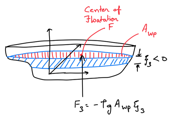
Note that the restoring force acts (upwards) in the direction opposite to the displacement (downward as \(\xi_3<0\)) and hence there is a minus sign in \(\eqref{eq-heave-heave-restoring}\). The corresponding force in the BCS is given by:
\[\begin{align} \begin{bmatrix} \tau_{hst,1} \\ \tau_{hst,2} \\ \tau_{hst,3} \end{bmatrix} = \boldsymbol{R}(\{\eta_{2m}\})^T\begin{bmatrix} 0 \\ 0 \\ F_3 \end{bmatrix} = \begin{bmatrix} -s_{2m} \\ s_{1m} c_{2m} \\ c_{1m} c_{2m} \end{bmatrix} F_3 \end{align}\]
Keeping terms upto the linear order leads to:
\[\begin{align} \begin{bmatrix} \tau_{hst,1} \\ \tau_{hst,2} \\ \tau_{hst,3} \end{bmatrix} = -\rho g A_{WP} \begin{bmatrix} 0 \\ 0 \\ 1 \end{bmatrix} \xi_3 \end{align}\]
This additional buoyancy force acts at the centroid of the additional volume of water displaced. For a small displacement \(\xi_3\), this centroid is equivalent to the centroid of the waterplane area. The centroid of the waterplane area is known as the center of floatation \(F\). Note that center of floatation \(F\) will in general will not coincide with the origin of the BCS and hence there will be a moment due to this force. If the location of \(F\) in BCS is given by \(\vec{r}_F = (x_F, y_F, z_F)\), then the restoring moment is given by:
\[\begin{align} \begin{bmatrix} \tau_{hst,4} \\ \tau_{hst,5} \\ \tau_{hst,6} \end{bmatrix} = \vec{r}_F \times \boldsymbol{R}(\{\eta_{2m}\})^T\begin{bmatrix} 0 \\ 0 \\ F_3 \end{bmatrix} = -\rho g A_{WP} \begin{bmatrix} y_F \\ - x_F \\ 0 \end{bmatrix} \xi_3 \end{align}\]
Thus the generalized hydrostatic force vector is given by:
\[\begin{align} \begin{bmatrix} \tau_{hst,1} \\ \tau_{hst,2} \\ \tau_{hst,3} \\ \tau_{hst,4} \\ \tau_{hst,5} \\ \tau_{hst,6} \end{bmatrix} = -\rho g A_{WP} \begin{bmatrix} 0 \\ 0 \\ 1 \\ y_F \\ - x_F \\ 0 \end{bmatrix} \xi_3 \end{align}\]
If the orientation of the BCS axis with respect the body is chosen in such a way that in the mean equilibruim position the vessel has zero roll and pitch angles \((\phi_m = \theta_m = 0)\), then the hydrostatic generalized force vector due to heave displacement reduces to:
\[\begin{align} \begin{bmatrix} \tau_{hst,1} \\ \tau_{hst,2} \\ \tau_{hst,3} \\ \tau_{hst,4} \\ \tau_{hst,5} \\ \tau_{hst,6} \end{bmatrix} = \begin{bmatrix} 0 \\ 0 \\ 1 \\ y_F \\ - x_F\\ 0 \end{bmatrix} F_3 = -\rho g A_{WP} \begin{bmatrix} 0 \\ 0 \\ 1 \\ y_F \\ -x_F \\ 0 \end{bmatrix} \xi_3 \end{align}\]
Defining \(I_x^A = \iint_{A_{WP}} x dA\) and \(I_y^A = \iint_{A_{WP}} y dA\), the generalized force reduces to:
\[\begin{align} \begin{bmatrix} \tau_{hst,1} \\ \tau_{hst,2} \\ \tau_{hst,3} \\ \tau_{hst,4} \\ \tau_{hst,5} \\ \tau_{hst,6} \end{bmatrix} = - \rho g \begin{bmatrix} 0 \\ 0 \\ A_{WP} \\ I_y^A \\ -I_x^A\\ 0 \end{bmatrix} \xi_3 \end{align}\]
6.3.2 Restoring Force and Moment due to Pitch/Roll Displacements
Consider a freely floating body as shown in Figure 6.2 (a) that is displaced in pitch by \(\xi_5>0\). Note that here it is assumed that the BCS is chosen in such a way that \(\phi_m = \theta_m = 0\). The small pitch displacement will change the instantaneous underwater volume by \(\Delta V = \iint_{A_{WP}} x \xi_5 dA = I_x^A \xi_5\) where \(I_x^A = \iint_{A_{WP}} x dA = x_F A_{WP}\). If the pitch displacement is small then the net restoring force acting on the body can be expressed as:
\[\begin{align} F_3 = \rho g \iint_{A_{WP}} x \xi_5 dA = \rho g x_F A_{WP} \xi_5 = \rho g I_x^A \end{align}\]
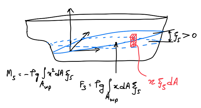
The corresponding moment generated by this additional buoyancy can be expressed as:
\[\begin{align} M_5 = - \rho g \iint_{A_{WP}} x^2 \xi_5 dA = - \rho g \nabla BM_L \xi_5 \end{align}\]
where \(BM_L\) is the longitudinal metacentric radius given by:
\[\begin{align} BM_L = \frac{\iint_{A_{WP}} x^2 dA}{\nabla} = \frac{I_{xx}^A}{\nabla} \end{align}\]
Note that \(I_{xx}^A\) is the second moment of inertia of the waterplane area.
An easy way to understand the sign in the above equations is to consider that case where the body coordinate system is located at the aft end of the vessel. A positive pitch will increase the underwater volume that will result in a positive heave force (upwards). However, this heave force will generate a negative pitch moment (opposing the applied pitch displacement).
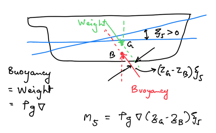
The above analysis has accounted for the forces and moments due to the change in underwater volume. However, one effect is still unaccounted for. The center of gravity \(G\) (with coordinates \((x_G, y_G, z_G)\)) and the center of buoyancy \(B\) (with coordinates \((x_B, y_B, z_B)\)) in a freely floating equilibrium must be in the same vertical line. When the body is pitched, this will no longer be true as shown in Figure 6.2 (b). Therefore the weight and static buoyancy forces will generate pitch moments. This additional pitch moment is given by:
\[\begin{align} M_5 = \rho g \nabla (z_G - z_B) \xi_5 = - \rho g \nabla (KB - KG) \xi_5 \end{align}\]
where \(K\) is the keel of the ship and \(KG\) and \(KB\) refer to the height of the center of gravity and center of buoynacy from the keel respectively. Thus the total pitch moment is given by:
\[\begin{align} M_5 = - \rho g \nabla (BM_L + KB - KG) \xi_5 = - \rho g \nabla GM_L \xi_5 \end{align}\]
Note that \(GM_L\) is known as the longitudinal metacentric height of the vessel. The roll moment caused by this pitch displacement can be calculated as:
\[\begin{align} M_4 = \rho g \iint_{A_{WP}} x y dA \xi_5 = \rho g I_{xy}^A \xi_5 \end{align}\]
where \(I_{xy}^A\) is the cross moment of inertia of the waterplane area. Note that for a ship with port-starboard symmetry \(I_{xy}^A = 0\). The generalized force vector for a small pitch displacement is given by:
\[\begin{align} \begin{bmatrix} \tau_{hst,1} \\ \tau_{hst,2} \\ \tau_{hst,3} \\ \tau_{hst,4} \\ \tau_{hst,5} \\ \tau_{hst,6} \end{bmatrix} = -\rho g\begin{bmatrix} 0 \\ 0 \\ -I_x^A \\ -I_{xy}^A \\ \nabla GM_L\\ 0 \end{bmatrix} \xi_5 \end{align}\]
A similar analysis for a small roll displacement \(\xi_4\) will result in a generalized force vector given by:
\[\begin{align} \begin{bmatrix} \tau_{hst,1} \\ \tau_{hst,2} \\ \tau_{hst,3} \\ \tau_{hst,4} \\ \tau_{hst,5} \\ \tau_{hst,6} \end{bmatrix} = -\rho g\begin{bmatrix} 0 \\ 0 \\ I_y^A \\ \nabla GM_T\\ -I_{xy}^A \\ 0 \end{bmatrix} \xi_4 \end{align}\]
where \(GM_T\) is the transverse metacentric height of the vessel.
6.3.3 Interactive Simulation: Where the \(G\)-\(B\) Moment Comes From
The step that most often causes difficulty is the second one above — the claim that the weight and the buoyancy generate a pitch moment \(\rho g \nabla (z_G - z_B) \xi_5\) once the body is displaced. The buoyancy still equals the weight, so why should two equal and opposite forces produce a moment at all?
The resolution is a matter of which frame you draw the picture in. The weight and the buoyancy are always vertical in the GCS — gravity does not tilt when the ship tilts, and neither does the direction in which pressure pushes the hull up. What the pitch displacement does is carry the points \(G\) and \(B\) around with the body. Two forces that are equal, opposite and vertical produce zero net force but a non-zero couple as soon as their lines of action are separated, and after a rotation \(\xi_5\) the points \(G\) and \(B\) — which started on one vertical line — are separated horizontally by \((z_G - z_B)\xi_5\). That horizontal separation is the lever, and \(\rho g \nabla\) is the force, which is exactly the moment quoted above.
Figure 6.2 (b) draws this in the BCS, with the hull upright and the arrows tilted. That is a perfectly correct picture, but it hides the mechanism, because in it the forces look as though they have rotated. Use the frame toggle in the tool below to switch the same instant between the two views:
- GCS view — the water is level, the hull is heeled, and both arrows are drawn strictly vertical. The lever between the two lines of action is directly visible.
- BCS view — the hull is upright and the waterline is tilted, so the arrows now appear to lean. This reproduces Figure 6.2 (b).
Nothing physical changes between the two; only the frame changes. Switching back and forth is the quickest way to see that the \(G\)-\(B\) moment is not an extra assumption but an unavoidable consequence of rotating the body under two vertical forces.
The tool also separates the two contributions that add up to \(GM\), and connects both of them to the waterplane integrals of the previous sections:
- The wedge term \(-\rho g \nabla BM_L \xi_5\) comes from the emerged and immersed wedges (shaded red and blue in the section view). Its size is set by \(I_{xx}^A = \iint_{A_{WP}} x^2 dA\), which is why the plan view shades each strip of the waterplane by its contribution to that integral. This term shifts \(B\) sideways to \(B'\).
- The \(G\)-\(B\) couple \(-\rho g \nabla (KB - KG)\xi_5\) comes from the vertical separation of \(G\) and \(B\), and does not involve the waterplane at all. Raise \(KG\) above \(KB\) and watch this term change sign.
Two distinct points are marked in the section view, and it is worth being clear about the difference between them. The BCS origin \(O\) (black crosshair) is the point the rotation \(\xi_5\) is defined about: the hull turns bodily about \(O\), and the arc labelled \(\xi_5\) is drawn there. The centre of flotation \(F\) (purple ring) is the centroid of the waterplane, and it is the point the waterline tips about, because \(F\) is the one point of the waterplane whose immersion is unchanged to first order. For the rectangular barge the two coincide and the distinction is invisible; select the ship-like or wedge waterplane and they separate visibly, since \(x_F = I_x^A / A_{WP} \ne 0\). That separation is precisely what the \(I_x^A\) entries of the stiffness matrix are keeping track of — they are the terms coupling heave to pitch, and they vanish only when \(O\) is placed at \(F\).
Switch each term off in turn to see how much of the restoring moment it is responsible for. Note that the wedge term is always stabilising, whereas the \(G\)-\(B\) term is stabilising only when \(G\) lies below \(B\); for a real ship \(G\) is almost always above \(B\), so the \(G\)-\(B\) term is destabilising and the vessel is stable only because the wedge term is larger. Raising \(KG\) far enough drives \(GM_T\) negative and the vessel becomes unstable — try the wedge hull at a high \(KG\) in roll.
Finally, the stiffness matrix \(\boldsymbol{C}\) of the next section is assembled live at the bottom of the tool. The column being excited is highlighted in yellow. The entries shaded red are the coupling terms \(I_x^A\), \(I_y^A\) and \(I_{xy}^A\): these vanish for a hull whose waterplane is symmetric about the BCS origin, and the asymmetry slider bends the waterplane off the centreline so you can watch \(I_{xy}^A\) — and with it the roll-pitch coupling \(C_{45} = C_{54}\) — switch on.
Weight \(W = \rho g \nabla\) through \(G\)
Buoyancy \(F_B = \rho g \nabla\) through \(B\)
Wedge shift \(B \rightarrow B'\)
\(O\) — BCS origin, the point the rotation is about
\(F\) — centre of flotation, the point the waterline tips about
Section view — the lever between the two lines of action
Waterplane — the source of the wedge term
1. Wedge (change of underwater volume)
Set by the waterplane inertia. Always stabilising.
2. \(G\)-\(B\) couple (two vertical forces, offset lines of action)
Total restoring moment
Negative opposes the displacement, so the vessel is stable.
\(A_{WP}\) m²
\(I_x^A = \iint x\,dA\) m³
\(I_y^A = \iint y\,dA\) m³
\(I_{xx}^A = \iint x^2 dA\) m⁴
\(I_{yy}^A = \iint y^2 dA\) m⁴
\(I_{xy}^A = \iint xy\,dA\) m⁴
\(\nabla\) m³
\(x_F\) m
\(KB\) m
\(= I/\nabla\) m
m
Yellow: the column being excited. Red: coupling entries that exist only
when the waterplane is asymmetric about the BCS origin.
6.3.4 Generalized Restoring Forces and Moments
Combining the generalized force vectors from heave, roll and pitch motions yields the generalized force vector that can be expressed as a matrix multiplication of the stiffness matrix \(\boldsymbol{C}\) with the displacement vector \(\{\xi\}\) as shown below:
\[\begin{align} \{\tau_{hst}\} = -\rho g\begin{bmatrix} 0 & 0 & 0 & 0 & 0 & 0 \\ 0 & 0 & 0 & 0 & 0 & 0 \\ 0 & 0 & A_{WP} & I_y^A & -I_x^A & 0 \\ 0 & 0 & I_y^A & \nabla GM_T & -I_{xy}^A & 0 \\ 0 & 0 & -I_x^A & -I_{xy}^A & \nabla GM_L & 0 \\ 0 & 0 & 0 & 0 & 0 & 0 \\ \end{bmatrix} \begin{bmatrix} \xi_1 \\ \xi_2 \\ \xi_3 \\ \xi_4 \\ \xi_5 \\ \xi_6 \end{bmatrix} = -\boldsymbol{C} \{\xi\} \end{align}\]
The stiffness matrix \(\boldsymbol{C}\) is given by:
\[\begin{align} \boldsymbol{C} = \rho g \begin{bmatrix} 0 & 0 & 0 & 0 & 0 & 0 \\ 0 & 0 & 0 & 0 & 0 & 0 \\ 0 & 0 & A_{WP} & I_y^A & -I_x^A & 0 \\ 0 & 0 & I_y^A & \nabla GM_T & -I_{xy}^A & 0 \\ 0 & 0 & -I_x^A & -I_{xy}^A & \nabla GM_L & 0 \\ 0 & 0 & 0 & 0 & 0 & 0 \\ \end{bmatrix} \end{align}\]
6.4 Hydrodynamic Forces and Moments in Calm Waters
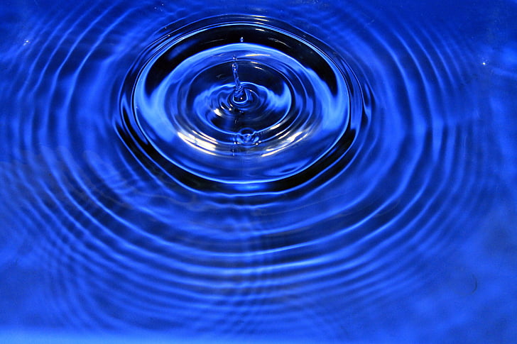
When a pebble is dropped into a calm water body, the water surface is disturbed and ripples are formed as shown in Figure 6.3. Similar waves are also produced when a floating body is moved from its equilibrium position on an initially calm water surface. These waves generated by the motion of the body are known as radiated waves. The force acting on the body due to these waves is known as the radiation force. Whenever a floating body experiences dynamic motion, waves are radiated and the body experiences the radiation force.
A structure in a dynamic fluid medium experiences two types of stress on its surface:
- Normal stress known as the pressure \(p\)
- Stress due to viscosity \(\boldsymbol{\tau} \hat{n}\)
Note that the normal stress due to pressure only acts perpendicular to the local surface. On the contrary the viscous stress has all three components - both the normal as well as two orthogonal tangential components with \(\boldsymbol{\tau}\) being a tensor defined as:
\[\begin{align} \boldsymbol{\tau} = \begin{bmatrix} \tau_{xx} & \tau_{xy} & \tau_{xz} \\ \tau_{yx} & \tau_{yy} & \tau_{yz} \\ \tau_{zx} & \tau_{zy} & \tau_{zz} \end{bmatrix} = \mu \begin{bmatrix} 2\frac{\partial u_1}{\partial x} & \left(\frac{\partial u_1}{\partial y} + \frac{\partial u_2}{\partial x}\right) & \left(\frac{\partial u_1}{\partial z} + \frac{\partial u_3}{\partial x}\right) \\ \left(\frac{\partial u_2}{\partial x} + \frac{\partial u_1}{\partial y}\right) & 2\frac{\partial u_2}{\partial y} & \left(\frac{\partial u_2}{\partial z} + \frac{\partial u_3}{\partial x}\right) \\ \left(\frac{\partial u_3}{\partial x} + \frac{\partial u_1}{\partial z}\right) & \left(\frac{\partial u_3}{\partial y} + \frac{\partial u_2}{\partial y}\right) & 2\frac{\partial u_3}{\partial z} \end{bmatrix} \end{align}\]
The net force on the structure is obtained by integrating the pressure and the wall shear stress across the surface \(S\) of the structure exposed to the fluid as shown below:
\[\begin{align} \vec{F} = \iint_S p\hat{n} dS - \iint_S \boldsymbol{\tau}\hat{n} dS \end{align}\]
where \(\hat{n}\) is the vector normal to the body surface pointing out of the fluid.
6.4.1 Dimensional Analysis of Viscous and Pressure Forces
A floating body oscillating in a calm water produces waves of the similar length as the characteristic length of the body \(L\). Assuming that the wavelength \(\lambda \sim L\) and an amplitude \(a\), the order of the pressure due to a wave can be estimated as
\[\begin{align} p \sim \rho g a \end{align}\]
The order of force acting on the body due to this pressure around the hull can be estimated as
\[\begin{align} F_p \sim \rho g a L^2 \end{align}\]
Now let’s consider the viscous forces. At the hull boundary, the order of the wall shear stress is given by
\[\begin{align} \boldsymbol{\tau} \sim \mu \frac{U}{\delta} \end{align}\]
where \(U\) is the characteristic velocity and \(\delta\) is the boundary layer thickness. The order of the viscous force is given by
\[\begin{align} F_v \sim \tau L^2 \sim \mu \frac{U}{\delta} L^2 \end{align}\]
A water particle in a wave experiences an orbital velocity \(U \sim a \omega\). Thus the ratio of the viscous to pressure forces can be estimated as
\[\begin{align} \frac{F_v}{F_p} \sim \frac{\mu \omega}{\rho g \delta} \sim \frac{\nu \omega}{g \delta} \label{eq-visc-pres-ratio} \end{align}\]
where \(\nu\) is the kinematic viscosity of the water. The order of the boundary layer thickness can also be estimated by considering force balance inside the boundary layer. Consider a fluid velocity parallel to a flat plate is oscillating with
\[\begin{align} u_1 = u_1(t, y) \end{align}\]
where the flat plate is assumed to be in the \(x\)-\(z\) plane and \(y\) is the direction normal to the surface. Neglecting the pressure gradient and the nonlinear convective terms, the \(x\)-momentum equation in the boundary layer can be assumed to be given by
\[\begin{align} \frac{\partial u_1}{\partial t} = \nu \frac{\partial^2 u_1}{\partial y^2} \end{align}\]
Considering the order of the terms, this can be approximated for an order of magnitude comparison as:
\[\begin{align} \frac{U}{1/\omega} \sim \nu \frac{U}{\delta^2} \end{align}\]
Rearranging, we can estimate the order the boundary layer thickness \(\delta\) as
\[\begin{align} \delta \sim \sqrt{\frac{\nu}{\omega}} \end{align}\]
Substituting this in \(\eqref{eq-visc-pres-ratio}\) yeilds:
\[\begin{align} \frac{F_v}{F_p} \sim \frac{\nu \omega}{g \delta} \sim \frac{\nu^{1/2}\omega^{3/2}}{g} \end{align}\]
Consider a ship of length \(100\) meters generating radiated waves of same length. The frequency of this wave can be estimated from the deep water dispersion relationship \(\omega = \sqrt{gk} \approx 0.79~rad/s\). Taking the sea water kinematic viscosity as \(\nu \approx 10^{-6} ~m^2/s\) yields:
\[\begin{align} \frac{F_v}{F_p} \sim \frac{\nu^{1/2}\omega^{3/2}}{g} \approx 10^{-5} \end{align}\]
It can be seen that viscous forces are five orders of magnitude smaller than the pressure forces. Therefore, for the seakeeping analysis, the force on the body is contributed primarily by the pressure term and therefore the fluid can be assumed to be inviscid.
\[\begin{align} \vec{F} = \iint_S p \hat{n} dS \label{eq-pressure-integration} \end{align}\]
6.4.2 Potential Flow
Consider a hull moving steadily with design speed \(U\) in calm waters. We will define a global coordinate system moving steadily forward along its \(x\)-axis with design speed \(U\). Assume that the BCS is also aligned with the GCS in the steady equilibrium condition \((\phi_m = \theta_m = \psi_m = 0)\). When dealing with a floating offshore structure, the design speed \(U=0\). For an inviscid flow, the momentum conservation equations for the fluid flow are given by the Euler equations (Navier Stokes equations with no viscosity):
\[\begin{align} \rho \left(\frac{\partial \vec{V}}{\partial t} + (\vec{V}.\nabla)\vec{V}\right) = -\nabla p + \rho \vec{g} \end{align}\]
where \(\vec{V}\) is the velocity of the fluid in the steadily moving GCS frame. For an offshore structure, the GCS will be stationary. For constant density (incompressible flow), this reduces to
\[\begin{align} \frac{\partial \vec{V}}{\partial t} + (\vec{V}.\nabla)\vec{V} = -\frac{\nabla p}{\rho} - g\nabla z \end{align}\]
Using the vector identity,
\[\begin{align} (\vec{V}.\nabla)\vec{V} = \nabla \left(\frac{|\vec{V}|^2}{2}\right) - \vec{V} \times (\nabla \times \vec{V}) \end{align}\]
the Euler’s equations can be recast as
\[\begin{align} \frac{\partial \vec{V}}{\partial t} + \nabla \left(\frac{|\vec{V}|^2}{2} + \frac{p}{\rho} + g z\right) = \vec{V} \times \vec{\Omega} \label{eq-euler-recast} \end{align}\]
where \(\vec{\Omega}\) is the vorticity. If the flow is irrotational, then \(\vec{\Omega} = 0\) and a total velocity potential \(\Phi\) can be defined as:
\[\begin{align} \vec{V} = \nabla\Phi = - U\hat{i}_0 + \nabla \varphi \label{eq-velocity-potential-def} \end{align}\]
where \(\varphi\) is the disturbance potential and corresponds to the velocity component of the fluid relative to the steady motion of GCS. Substituting this into \(\eqref{eq-euler-recast}\) results in
\[\begin{align} \nabla \left(\frac{\partial \Phi}{\partial t} + \frac{1}{2}\left|\nabla\Phi\right|^2 + \frac{p}{\rho} + g z\right) = 0 \end{align}\]
Expressing in terms of disturbance potential \(\varphi\) results in:
\[\begin{align} \nabla \left(\frac{\partial \varphi}{\partial t} - U \frac{\partial \varphi}{\partial x} + \frac{1}{2}\left|\nabla\varphi\right|^2 + \frac{p}{\rho} + g z\right) = 0 \end{align}\]
This means that the quantity inside the gradient can depend only on time:
\[\begin{align} \frac{\partial \varphi}{\partial t} - U \frac{\partial \varphi}{\partial x} + \frac{1}{2}\left|\nabla\varphi\right|^2 + \frac{p}{\rho} + g z = C(t) \label{eq-bernoulli-unsteady} \end{align}\]
and this expression is known as the unsteady Bernoulli’s equation. The conservation of mass for an incompressible, inviscid flow is given by the continuity equation shown below.
\[\begin{align} \nabla.\vec{V} = 0 \end{align}\]
If the flow is irrotational, a velocity potential \(\varphi\) is defined and the continuity equation reduces to the Laplace equation as shown below:
\[\begin{align} \nabla.\vec{V} = \nabla.(-U\hat{i}_0 + \nabla \varphi) = \nabla^2 \varphi = 0 \label{eq-laplace} \end{align}\]
The Euler’s equations and the continuity equation describe the fluid flow using four equations with four unknowns - pressure \(p\) and three velocities \(u_1\), \(u_2\) and \(u_3\). Under the assumptions of inviscid, incompressible and irrotational flow, a velocity potential \(\varphi\) is admitted that reduces the problem to one governing Laplace equation. Note that the velocities \(u_1\), \(u_2\) and \(u_3\) can be obtained from the gradient of the velocity potential \(\nabla \varphi\) as seen in \(\eqref{eq-velocity-potential-def}\) and the pressure \(p\) is obtained from the unsteady Bernoulli’s equation \(\eqref{eq-bernoulli-unsteady}\).
6.4.3 Boundary Value Problem
In order to compute the hydrodynamic force acting on the body due to the radiated waves generated due to the body motion, we need to know the pressure acting on the hull wetted surface area. If the pressure is known, then it can be integrated to obtain the hydrodynamic force and moment acting on the vessel as seen in \(\eqref{eq-pressure-integration}\). As we have seen, the pressure can be obtained from the Bernoulli’s equation \(\eqref{eq-bernoulli-unsteady}\) if we know the velocity potential \(\varphi\) generated due to the body motion in calm waters. Therefore, the governing Laplace equation \(\eqref{eq-laplace}\) needs to be solved inside the fluid domain to calculate the hydrodynamic force and moment acting on the vessel.
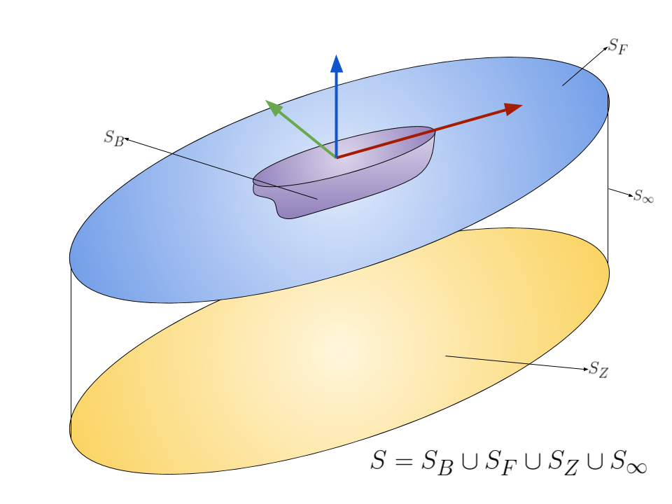
The fluid domain is bounded by the free surface \(S_F\), body boundary \(S_B\) (wetted surface area of the hull), bottom boundary \(S_Z\) and the vertical boundary \(S_{\infty}\) located at an infinite radial distance away from the hull. In order to solve the governing Laplace equation shown in \(\eqref{eq-laplace}\) and obtain the flow parameters inside the domain, we need to impose the boundary conditions on these fluid boundaries.
Kinematic Free Surface Boundary Condition
Consider a particle on the disturbed free surface (due to radiated waves). Let the particle’s position in GCS be denoted by \(\vec{r}_{P}(t) = (x_{P}(t), y_{P}(t), z_{P}(t))\) and let its velocity in GCS be given by \(\vec{V} = (-U + u_1, u_2, u_3)\).
\[\begin{align} \vec{V} = \frac{d}{dt} \vec{r}_{P}(t) \end{align}\]
Let the disturbed free surface be denoted by \(S_F(x, y, z, t) = 0\). However, the particle’s position itself is also time dependent and can explicitly be written as:
\[\begin{align} S_F(x_{P}(t), y_{P}(t), z_{P}(t), t) = 0 \end{align}\]
Therefore, the time derivative of the free surface can be computed using the chain rule of differentiation as:
\[\begin{align} \frac{d S_F}{dt} &= \frac{\partial S_F}{\partial t} + \frac{\partial S_F}{\partial x} \frac{\partial x_P}{\partial t} + \frac{\partial S_F}{\partial y} \frac{\partial y_P}{\partial t} + \frac{\partial S_F}{\partial z} \frac{\partial z_P}{\partial t} \nonumber \\ &= \frac{\partial S_F}{\partial t} + (-U + u_1) \frac{\partial S_F}{\partial x} + u_2 \frac{\partial S_F}{\partial y} + u_3 \frac{\partial S_F}{\partial z} \nonumber \\ &= \left[\frac{\partial}{\partial t} + (\vec{V}.\nabla)\right] S_F \end{align}\]
This operator on the right hand side is also known as the material derivative and is denoted as:
\[\begin{align} \frac{D}{Dt} = \left[\frac{\partial}{\partial t} + (\vec{V}.\nabla)\right] \end{align}\]
Since the free surface is a material surface (a surface made up of the same fluid particles as time evolves), a fluid particle that is initially on the free surface remains on the free surface. If \(S_F(x_P(t_0), y_P(t_0), z_P(t_0), t_0) = 0\) then \(S_F(x_P(t), y_P(t), z_P(t), t) = 0\) for all \(t\). Therefore,
\[\begin{align} \frac{d}{dt} S_F(x_P(t), y_P(t), z_P(t), t) = 0 \end{align}\]
which gives the kinematic free surface boundary condition:
\[\begin{align} \frac{DS_F}{Dt} = \left[\frac{\partial}{\partial t} + (\vec{V}.\nabla)\right] S_F = 0 \end{align}\]
Let the wave elevation be denoted by the function \(\eta(x, y, t)\) defined as the height of the free surface from \(z=0\). The free surface \(S_F\) can then be described as:
\[\begin{align} S_F(x, y, z, t) = z - \eta(x, y, t) \end{align}\]
The kinematic free surface boundary condition can be evaluated as:
\[\begin{align} &\left[\frac{\partial}{\partial t} + (\vec{V}.\nabla)\right] (z - \eta) = 0 \nonumber\\ &u_3 - \frac{\partial \eta}{\partial t} - (-U + u_1) \frac{\partial \eta}{\partial x} - u_2 \frac{\partial \eta}{\partial y} = 0 \nonumber\\ &\frac{\partial \varphi}{\partial z} - \frac{\partial \eta}{\partial t} - \left(-U + \frac{\partial \varphi}{\partial x}\right) \frac{\partial \eta}{\partial x} - \frac{\partial \varphi}{\partial y} \frac{\partial \eta}{\partial y} = 0 \end{align}\]
Thus the kinematic free surface boundary condition is given by:
\[\begin{align} \frac{\partial \eta}{\partial t} - U\frac{\partial \eta}{\partial x} + \frac{\partial \varphi}{\partial x} \frac{\partial \eta}{\partial x} + \frac{\partial \varphi}{\partial y} \frac{\partial \eta}{\partial y} - \frac{\partial \varphi}{\partial z} = 0 \text{ over } z = \eta(x, y, t) \end{align}\]
Notice here that the kinematic boundary condition is applied on the unknown free surface \(z = \eta(x, y, t)\).
Dynamic Free Surface Boundary Condition
This is a second boundary condition imposed on the free surface that the pressure at the interface is equal to the atmospheric pressure \(p_{atm}\). Applying the Bernoulli’s equation on the free surface \(S_F = z - \eta = 0\) yeilds
\[\begin{align} \frac{\partial \varphi}{\partial t} - U \frac{\partial \varphi}{\partial x} + \frac{1}{2}\left|\nabla\varphi\right|^2 + \frac{p_{atm}}{\rho} + g \eta = C(t) \end{align}\]
Without loss of generality, \(C(t)\) can be chosen to be equal to \(p_{atm}/\rho\) so that the dynamic free surface boundary condition is given by:
\[\begin{align} \frac{\partial \varphi}{\partial t} - U \frac{\partial \varphi}{\partial x} + \frac{1}{2}\left|\nabla\varphi\right|^2 + g \eta = 0 \text{ over } z = \eta(x, y, t) \end{align}\]
Vanishing right hand side of Bernoulli’s equation
We have the flexibility to define a new potential \(\tilde{\varphi}\) as
\[\begin{align} \tilde{\varphi} = \varphi - f(t) \end{align}\]
where \(f(t)\) is an arbitrarily chosen function. The partial derivative with time then becomes:
\[\begin{align} \frac{\partial \tilde{\varphi}}{\partial t} = \frac{\partial \varphi}{\partial t} - \frac{df}{dt}(t) \end{align}\]
Notice that the velocity \(\nabla \tilde{\varphi} = \nabla \varphi\) remains unchanged. Therefore, \(f(t)\) can be chosen such that the right hand side of the unsteady Bernoulli’s equation vanishes. Thus the dynamic free surface boundary condition is commonly written as:
\[\begin{align} \frac{\partial \varphi}{\partial t} - U \frac{\partial \varphi}{\partial x} + \frac{1}{2}\left|\nabla\varphi\right|^2 + g \eta = 0 \text{ over } z = \eta(x, y, t) \end{align}\]
Bottom Boundary Condition
At the seabed the imposed condition is that no penetration condition. This means that the fluid should have no normal velocity at the seabed. This is specified mathematically as:
\[\begin{align} \frac{\partial \varphi}{\partial z} = 0 \text{ over } z = -h \end{align}\]
If we are dealing ships and offshore structures operating in deep waters, then this condition is imposed on \(z=-\infty\).
Radiation Boundary Condition
At the infinite boundary \(S_{\infty}\), the waves generated from the body must be propagating outwards towards the infinite boundary. This is enforced by applying the Sommerfield radiation boundary condition on \(S_{\infty}\):
\[\begin{align} \lim_{r\rightarrow\infty} \sqrt{r}\left[\frac{\partial \varphi}{\partial r} - i k \varphi\right] = 0 \end{align}\]
where \(r = \sqrt{x^2 + y^2}\) is the radial horizontal distance and \(k\) is the wavenumber of the outgoing wave.
Body Boundary Condition
This is the most crucial boundary condition as it related the rigid body motion to the hydrodynamic boundary value problem. Since we are now dealing with inviscid flow (as viscous effects are negligible) the boundary condition imposed on the hull boundary is no penetration boundary condition. This is similar to the bottom boundary but with the difference that the boundary is moving. Mathematically the body boundary condition can be specified as:
\[\begin{align} (\vec{V}_s - \nabla \Phi).\hat{n} = 0 \text{ over } S_B(t) \end{align}\]
over the instantaneous underwater surface \(S_B(t)\). Note that \(\vec{V}_s\) represents the local velocity on the ship hull and differs from point to point as the vessel experiences both translational velocity \(\dot{\vec{\xi}}_{t} = \begin{bmatrix}\dot{\xi}_1 & \dot{\xi}_1 & \dot{\xi}_3 \end{bmatrix}^T\) as well as angular velocity \(\dot{\vec{\xi}}_{r} = \begin{bmatrix}\dot{\xi}_4 & \dot{\xi}_5 & \dot{\xi}_6 \end{bmatrix}^T\). Here we are making use of the assumption of small amplitude of motion and velocity. Expanding in terms of the disturbance potential \(\varphi\) yeilds:
\[\begin{align} \frac{\partial \varphi}{\partial n} \equiv \nabla \varphi . \hat{n} = (\dot{\vec{\xi}}_{t} + \dot{\vec{\xi}}_{r} \times \vec{r}_{P}).\hat{n} - \nabla(-Ux).\hat{n} \text{ over } S_B(t) \end{align}\]
where \(\vec{r}_{P}\) denotes the vector from BCS origin to a point \(P\) on the underwater hull surface \(S_B(t)\). Note that \(\hat{n}\) represents the instantaneous normal at point \(P\) on the hull surface that changes with time due to the motion of the vessel.
Boundary Value Problem Summary
Summarizing the boundary value problem, the governing equation is given by:
\[\begin{align} \nabla^2 \varphi = 0 \end{align}\]
with the following boundary conditions:
\[\begin{align} \frac{\partial \eta}{\partial t} - U\frac{\partial \eta}{\partial x} + \frac{\partial \varphi}{\partial x} \frac{\partial \eta}{\partial x} + \frac{\partial \varphi}{\partial y} \frac{\partial \eta}{\partial y} - \frac{\partial \varphi}{\partial z} = 0 \text{ over } z = \eta(x, y, t) \end{align}\]
\[\begin{align} \frac{\partial \varphi}{\partial t} - U \frac{\partial \varphi}{\partial x} + \frac{1}{2}\left|\nabla\varphi\right|^2 + g \eta = 0 \text{ over } z = \eta(x, y, t) \end{align}\]
\[\begin{align} \frac{\partial \varphi}{\partial z} = 0 \text{ over } S_Z = z + h = 0 \end{align}\]
\[\begin{align} \lim_{r\rightarrow\infty} \sqrt{r}\left[\frac{\partial \varphi}{\partial r} - i k \varphi\right] = 0 \text{ over } S_{\infty} \end{align}\]
\[\begin{align} \frac{\partial \varphi}{\partial n} = (\dot{\vec{\xi}}_{t} + \dot{\vec{\xi}}_{r} \times \vec{r}_{P}).\hat{n} - \nabla(-Ux).\hat{n} \text{ over } S_B(t) \end{align}\]
Note that while the govering equation is linear, the free surface and body boundary conditions are not. The body boundary condition couples the motion of the rigid body strongly with the hydrodynamic problem. It is not possible to obtain an exact analytical closed form solution to this boundary value problem. In order to make the problem tenable, we will linearize the boundary conditions and use the principle of superposition (from Chapter 2 and Chapter 3) to separate the problem into 6 sub-problems.
Interactive Anatomy of the Boundary Value Problem
Figure 6.4 names the four boundaries; the tool below attaches the mathematics to each of them. Click a surface in the diagram — or a tab — to see the condition imposed there, what it physically asserts, and what happens to it under linearisation.
The Exact / Linearised toggle is the part worth spending time on. Switching between the two shows, boundary by boundary, precisely which terms perturbation theory throws away and, more importantly, where each condition is applied. Two observations that are easy to state but hard to see in a static figure:
- The governing equation is never linearised. Laplace’s equation is already linear, and every order of the perturbation series satisfies the identical equation. Select the fluid domain and toggle: nothing changes. All of the approximation in this chapter lives in the boundary conditions.
- Only two boundaries actually move, and they are exactly the two that cause trouble. The seabed and the far field are fixed, and their conditions pass through linearisation untouched. The free surface condition is imposed on the unknown surface \(z = \eta(x,y,t)\) and is moved to the known plane \(z=0\); the body condition is imposed on the instantaneous wetted surface \(S_B(t)\) and is moved to the mean surface \(S_{B0}\). Those two moves are what turn an intractable problem into six solvable ones.
6.4.4 Linearized Boundary Value Problem
As the nonlinear boundary value problem cannot be solved analytically, we employ an approach known as perturbation theory to separate the problem into a series of problems of increasing order of nonlinearity. The solution \(\varphi\) and other parameters of interest (wave elevation \(\eta\), pressure \(p\), normal vector \(\hat{n}\), position vector \(\vec{r}_P\), rigid body displacement \(\xi_k\) for \(k=1,2,...,6\)) are expressed as series expansion in terms of a small quantity \(\epsilon\) (usually of the order of wave slope).
\[\begin{align} \varphi &= \epsilon \varphi^{(1)} + \epsilon^2 \varphi^{(2)} + ~ ... \\ \eta &= \epsilon \eta^{(1)} + \epsilon^2 \eta^{(2)} + ~ ... \\ p &= p^{(0)} + \epsilon p^{(1)} + \epsilon^2 p^{(2)} + ~ ... \\ \hat{n} &= \hat{n}^{(0)} + \epsilon \hat{n}^{(1)} + \epsilon^2 \hat{n}^{(2)} + ~ ... \\ \vec{r}_P &= \vec{r}_P^{(0)} + \epsilon \vec{r}_P^{(1)} + \epsilon^2 \vec{r}_P^{(2)} + ~ ... \\ \xi_k &= \epsilon \xi_k^{(1)} + \epsilon^2 \xi_k^{(2)} + ~ ... \text{ for } k =1,2,...,6 \end{align}\]
Substituting this into the governing equation and the boundary conditions results in the problem being reduced to solving successive set of Laplace equations for each order of \(\epsilon\). The boundary value problem for \(\varphi^{(1)}\) is obtained by only keeping terms upto the first order of \(\epsilon\) and is given by:
\[\begin{align} \nabla^2 \varphi^{(1)} = 0 \end{align}\]
\[\begin{align} \frac{\partial \varphi^{(1)}}{\partial t} - U \frac{\partial \varphi^{(1)}}{\partial x} + g \eta = 0 \text{ over } z = 0 \end{align}\]
\[\begin{align} \frac{\partial \eta^{(1)}}{\partial t} - U\frac{\partial \eta^{(1)}}{\partial x} - \frac{\partial \varphi^{(1)}}{\partial z} = 0 \text{ over } z = 0 \end{align}\]
\[\begin{align} \frac{\partial \varphi^{(1)}}{\partial z} = 0 \text{ over } S_Z = z + h = 0 \end{align}\]
\[\begin{align} \lim_{r\rightarrow\infty} \sqrt{r}\left[\frac{\partial \varphi^{(1)}}{\partial r} - i k \varphi^{(1)}\right] = 0 \text{ over } S_{\infty} \end{align}\]
The body boundary condition when linearized yeilds
\[\begin{align} \frac{\partial \varphi^{(1)}}{\partial n} = \sum_{k=1}^{6} \dot{\xi}_k^{(1)} n_k + \xi_k^{(1)} m_k \text{ over } S_{B0} \end{align}\]
where
\[\begin{align} (n_1, n_2, n_3) &= \hat{n}^{(0)} \\ (n_4, n_5, n_6) &= \vec{r}_P^{(0)} \times \hat{n}^{(0)} \\ (m_1, m_2, m_3) &= -(\hat{n}^{(0)}.\nabla) \vec{W} \\ (m_4, m_5, m_6) &= -(\hat{n}^{(0)}.\nabla) (\vec{r}_P^{(0)} \times \vec{W}) \end{align}\]
\(\vec{W} = -U\hat{i}_0\) is the steady flow around the hull and \(S_{B0}\) is the surface of the hull in its equilibrium position \((\{\xi\} = 0)\). The linearized potential \(\varphi^{(1)}\) is the potential caused due to the small amplitude motion of the rigid body along the six degrees of freedom. However, since the boundary value problem is now linear, we can separate the potential into six components (one for each degree of freedom).
\[\begin{align} \varphi^{(1)} = \sum_{k=1}^{6} \tilde{\varphi}_k^{(1)} \label{eq-potential-superposition} \end{align}\]
Thus the same linearized boundary value problem can be solved for each of the \(\tilde{\varphi}_k^{(1)}\) for \(k=1,2,...,6\) with the boundary condition for each \(\tilde{\varphi}_k^{(1)}\) specified as:
\[\begin{align} \frac{\partial \tilde{\varphi}_k^{(1)}}{\partial n} = \dot{\xi}_k^{(1)} n_k + \xi_k^{(1)} m_k \text{ over } S_{B0} \end{align}\]
Notice that the rigid body motions \(\xi_k^{(1)}(t)\), even though of small amplitude, is coupled to the hydrodynamic problem. \(\tilde{\varphi}_k^{(1)}\) depends on \(\xi_k^{(1)}\) and viceversa. In order to separate the hydrodynamic and rigid body motion problems, we define the potential \(\varphi_k^{(1)}\) caused due to an impulsive displacement \(\xi_k^{(1)}(t) = \delta(t)\). The potential \(\tilde{\varphi}_k^{(1)}(t)\) for a generic \(\xi_k^{(1)}(t)\) can then be expressed in terms of a convolution integral as:
\[\begin{align} \tilde{\varphi}_k^{(1)}(t) = \int_{-\infty}^{t} \varphi_k^{(1)}(t-\tau) \xi_k^{(1)}(\tau) d\tau \end{align}\]
Taking a Fourier transform yields:
\[\begin{align} \hat{\tilde{\varphi}}_k^{(1)} (\omega) = \hat{\varphi}_k^{(1)}(\omega) \xi_k^{(1)}(\omega) \label{eq-impulsive-potential-fourier} \end{align}\]
In the frequency domain we deal with solving the boundary value problem only for a single frequency at a time. Taking a Fourier transform of the boundary value problem for \(\varphi^{(1)}\) and using \(\eqref{eq-potential-superposition}\) and \(\eqref{eq-impulsive-potential-fourier}\) yields the governing equation:
\[\begin{align} \nabla^2 \hat{\varphi}_k^{(1)} = 0 \end{align}\]
combined free surface boundary condition:
\[\begin{align} \left(i \omega - U \frac{\partial }{\partial x}\right)^2 \hat{\varphi}_k^{(1)} + g \frac{\partial \hat{\varphi}_k^{(1)}}{\partial z} = 0 \text{ over } z = 0 \end{align}\]
bottom boundary condition:
\[\begin{align} \frac{\partial \hat{\varphi}_k^{(1)}}{\partial z} = 0 \text{ over } S_Z = z + h = 0 \end{align}\]
radiation boundary condition:
\[\begin{align} \lim_{r\rightarrow\infty} \sqrt{r}\left[\frac{\partial \hat{\varphi}_k^{(1)}}{\partial r} - i k \hat{\varphi}_k^{(1)}\right] = 0 \text{ over } S_{\infty} \end{align}\]
and body boundary condition:
\[\begin{align} \frac{\partial \hat{\varphi}_k^{(1)}}{\partial n} = (i \omega n_k + m_k) \text{ over } S_{B0} \end{align}\]
where \(\hat{\varphi}_k^{(1)} = \mathcal{F}\left(\varphi_k^{(1)}\right)\). Note that by taking the Fourier transform of the linearized boundary value problem, an arbitrary small amplitude rigid body motion of the vessel has been separated into infinitely many sinusoidal motions at various continuous frequencies \(\omega\).
6.4.5 Solving Linearized Boundary Value Problem
There are different methods to solve the linearized boundary value problem described above. Some of the popular approaches include the boundary element methods and finite element methods. However, the boundary element methods have now emerged as the standard approach to solve this problem due to the advantages of only needing to mesh the fluid boundary (surface) instead of meshing the fluid domain (volume) as required by finite element methods. The discussion of the boundary element methods is beyond the purview of this course.
There are several software tools that have emerged over the years to solve this boundary value problem. Some of the common tools include WAMIT and ANSYS AQWA. My research group (suprisingly several undergraduate students have contributed to this project) has also developed a web application (HydRA) to solve this boundary value problem.
6.4.6 Calculating Hydrodynamic Forces and Moments
Once the linearized boundary value problem has been solved, the potential \(\hat{\varphi}_k^{(1)}\) is known. However, our interest is to calculate the forces and moments acting on the vessel. It was seen previously that the force on the vessel can be obtained by integrating the pressure across the hull. The generalized force \(\{F\}\) acting on the vessel can be evaluated as:
\[\begin{align} \{F\} = \begin{bmatrix} \vec{F} \\ \vec{M} \end{bmatrix} = \begin{bmatrix} \iint_S p \hat{n} dS \\ \iint_S p (\vec{r}_P \times \hat{n}) dS \end{bmatrix} = \text{ over } S_B(t) \end{align}\]
The pressure can be expressed in terms of the potential using the unsteady Bernoulli’s equation and the application of perturbation theory will allow the generalized force to be expressed in orders of \(\epsilon\).
\[\begin{align} \vec{F} &= \vec{F}^{(0)} + \epsilon\vec{F}^{(1)} + \epsilon^2\vec{F}^{(2)} + ~ ... \\ \vec{M} &= \vec{M}^{(0)} + \epsilon\vec{M}^{(1)} + \epsilon^2\vec{M}^{(2)} + ~ ... \end{align}\]
\[\begin{align} \vec{F} &= \iint_{S_B(t)} dS \left[-\rho \left(\frac{\partial \varphi}{\partial t} - U \frac{\partial \varphi}{\partial x} + \frac{1}{2}\left|\nabla\varphi\right|^2 + g z\right) \hat{n}\right] \\ &= \left(\iint_{S_{B0}} dS + \epsilon \iint_{S_{B1}} dS + ~ ...\right) \left[-\rho \left(\left(\frac{\partial }{\partial t} - U \frac{\partial }{\partial x}\right) (\epsilon\varphi^{(1)} + \epsilon^2 \varphi^{(2)} + ~ ...) \right.\right.\nonumber \\ & \quad \left.\left.+ \frac{1}{2}\left|\nabla(\epsilon\varphi^{(1)} + \epsilon^2 \varphi^{(2)} + ~ ...)\right|^2 + g (z^{(0)} + \epsilon z^{(1)} + \epsilon^2 z^{(2)} + ~ ...)\right) \right.\nonumber\\ & \quad \left. .(\epsilon\hat{n}^{(1)} + \epsilon^2 \hat{n}^{(2)} + ~ ...) \right] \end{align}\]
Note that we have expanded the instantaneous wetted surface \(S_B(t)\) into its perturbation series.
\[\begin{align} S_B(t) = S_{B0} + \epsilon S_{B1}(t) + ~ ... \end{align}\]
Collecting the terms by orders of \(\epsilon\) yields the zeroth order force and moments as:
\[\begin{align} \vec{F}^{(0)} &= \iint_{S_{B0}} - \rho g z^{(0)} \hat{n}^{(0)} dS \\ \vec{M}^{(0)} &= \iint_{S_{B0}} - \rho g z^{(0)} (\vec{r}_P^{(0)} \times \hat{n}^{(0)}) dS \\ \end{align}\]
It can be seen that this is just the integration of the hydrostatic pressure over the mean wetted surface area of the hull in its equilibrium position. For a vessel floating at even keel, the hydrostatic force \(\vec{F}^{(0)}\) is the buoyancy force in the equilibrium condition and \(\vec{M}^{(0)}\) is the moment of the buoyancy force about the BCS origin. The buoyancy force will be balanced by the weight and the moment will be balanced by the moment of the weight about the BCS origin. The first order forces and moments can be computed as:
\[\begin{align} \vec{F}^{(1)} &= \iint_{S_{B0}} - \rho \left(\left(\frac{\partial }{\partial t} - U \frac{\partial }{\partial x}\right)\varphi^{(1)} + g z^{(1)}\right) \hat{n}^{(0)} dS \nonumber\\ & \quad + \iint_{S_{B0}} - \rho g z^{(0)} \hat{n}^{(1)} dS + \iint_{S_{B1}} - \rho g z^{(0)} \hat{n}^{(0)} dS \\ \vec{M}^{(1)} &= \iint_{S_{B0}} - \rho \left(\left(\frac{\partial }{\partial t} - U \frac{\partial }{\partial x}\right)\varphi^{(1)} + g z^{(1)}\right) (\vec{r}_P^{(0)} \times \hat{n}^{(0)}) dS \nonumber\\ & \quad + \iint_{S_{B0}} - \rho g z^{(0)} (\vec{r}_P^{(0)} \times \hat{n}^{(1)}) dS + \iint_{S_{B0}} - \rho g z^{(0)} (\vec{r}_P^{(1)} \times \hat{n}^{(0)}) dS \nonumber\\ & \quad + \iint_{S_{B1}} - \rho g z^{(0)} (\vec{r}_P^{(0)} \times \hat{n}^{(0)}) dS \end{align}\]
\(S_{B1}\) is the first order variation of \(S_{B0}\) and the integral over this surface can be represented as:
\[\begin{align} \iint_{S_{B1}} (.) dS = \int_{WL0} \zeta_r^{(1)} (.) dl \end{align}\]
where \(WL0\) is the mean waterline of the vessel in its equilibrium position and \(\zeta_r^{(1)}\) is the first order relative waterlevel and is given by:
\[\begin{align} \zeta_r^{(1)} = \eta^{(1)} - \left(\xi_3^{(1)} - \xi_5^{(1)} x^{(0)} + \xi_4^{(1)} y^{(0)}\right) \end{align}\]
Note that \(z^{(0)} = 0\) on \(WL0\) and the first order force and moment contributions due to the integral over \(S_{B1}\) are zero.
\[\begin{align} \iint_{S_{B1}} &- \rho g z^{(0)} \hat{n}^{(0)} dS = 0 \\ \iint_{S_{B1}} &- \rho g z^{(0)} (\vec{r}_P^{(0)} \times \hat{n}^{(0)}) dS = 0 \end{align}\]
Note that \(z^{(1)}\) is the z-component of the vector \(\vec{r}_P^{(1)}\). Both the normal vector \(\hat{n}\) and the position vector of a point on the hull \(\vec{r}_P\) up to the first order are given by:
\[\begin{align} \vec{r}_P &= \vec{r}_P^{(0)} + \epsilon \left(\vec{\xi}_t^{(1)} + \vec{\xi}_r^{(1)} \times \vec{r}_P^{(0)}\right) + ~ ... \\ \hat{n} &= \hat{n}^{(0)} + \epsilon \left(\vec{\xi}_r^{(1)} \times \hat{n}^{(0)}\right) + ~ ... \end{align}\]
The expression for first order force and first order moment reduce to:
\[\begin{align} \vec{F}^{(1)} &= \vec{F}_{rad}^{(1)} + \vec{F}_{hst}^{(1)} \nonumber\\ &= - \rho\iint_{S_{B0}} \left(\frac{\partial }{\partial t} - U \frac{\partial }{\partial x}\right)\varphi^{(1)} \hat{n}^{(0)} dS \nonumber\\ & \quad - \rho g \iint_{S_{B0}} \left(z^{(1)} \hat{n}^{(0)} + z^{(0)} \hat{n}^{(1)}\right) dS \\ \vec{M}^{(1)} &= \vec{M}_{rad}^{(1)} + \vec{M}_{hst}^{(1)} \nonumber\\ &= - \rho \iint_{S_{B0}}\left(\frac{\partial }{\partial t} - U \frac{\partial }{\partial x}\right)\varphi^{(1)} (\vec{r}_P^{(0)} \times \hat{n}^{(0)}) dS \nonumber\\ & \quad - \rho g \iint_{S_{B0}} \left(z^{(1)} (\vec{r}_P^{(0)} \times \hat{n}^{(0)}) + z^{(0)} (\vec{r}_P^{(0)} \times \hat{n}^{(1)}) + z^{(0)} (\vec{r}_P^{(1)} \times \hat{n}^{(0)}) \right) dS \end{align}\]
In both the force and moment expressions above, the first integral corresponds to the hydrodynamic force or moment due to the radiated wave (depends on \(\varphi^{(1)}\)) and the second term corresponds to the hydrostatic force or moment discussed previously. It can be shown that the hydrostatic component is the same as derived before:
\[\begin{align} \begin{bmatrix} \vec{F}_{hst}^{(1)} \\ \vec{M}_{hst}^{(1)} \end{bmatrix} &= -\rho g \begin{bmatrix} 0 & 0 & 0 & 0 & 0 & 0 \\ 0 & 0 & 0 & 0 & 0 & 0 \\ 0 & 0 & A_{WP} & I_y^A & -I_x^A & 0 \\ 0 & 0 & I_y^A & \nabla GM_T & -I_{xy}^A & 0 \\ 0 & 0 & -I_x^A & -I_{xy}^A & \nabla GM_L & 0 \\ 0 & 0 & 0 & 0 & 0 & 0 \end{bmatrix} \begin{bmatrix} \xi_1 \\ \xi_2 \\ \xi_3 \\ \xi_4 \\ \xi_5 \\ \xi_6 \end{bmatrix} = -\boldsymbol{C} \{\xi\} \label{eq-hydrostatics-1} \end{align}\]
Thus the hydrodynamic force can be expressed as:
\[\begin{align} \vec{F}_{rad}^{(1)} &= - \rho\iint_{S_{B0}} \left(\frac{\partial }{\partial t} - U \frac{\partial }{\partial x}\right)\varphi^{(1)} \hat{n}^{(0)} dS \\ &= - \rho \sum_{k=1}^{6} \iint_{S_{B0}} \left(\frac{\partial }{\partial t} - U \frac{\partial }{\partial x}\right)\tilde{\varphi}_k^{(1)} \xi_k^{(1)} \hat{n}^{(0)} dS\\ \vec{M}_{rad}^{(1)} &= - \rho \iint_{S_{B0}} \left(\frac{\partial }{\partial t} - U \frac{\partial }{\partial x}\right)\varphi^{(1)} (\vec{r}_P^{(0)} \times \hat{n}^{(0)}) dS \\ &= - \rho \sum_{k=1}^{6} \iint_{S_{B0}} \left(\frac{\partial }{\partial t} - U \frac{\partial }{\partial x}\right)\tilde{\varphi}_k^{(1)} (\vec{r}_P^{(0)} \times \hat{n}^{(0)}) dS \end{align}\]
Taking a Fourier transform leads to:
\[\begin{align} \left\{\hat{\tau}_{rad}(\omega)\right\} = \begin{bmatrix} \hat{\vec{F}}_{rad}^{(1)} (\omega) \\ \hat{\vec{M}}_{rad}^{(1)} (\omega) \end{bmatrix} = -\rho \sum_{k=1}^{6} \begin{bmatrix} \iint_{S_{B0}} \left(i\omega - U \frac{\partial }{\partial x}\right)\hat{\varphi}_k^{(1)} \hat{\xi}_k^{(1)} \hat{n}^{(0)} dS \\ \iint_{S_{B0}} \left(i\omega - U \frac{\partial }{\partial x}\right)\hat{\varphi}_k^{(1)} \hat{\xi}_k^{(1)} (\vec{r}_P^{(0)} \times \hat{n}^{(0)}) dS \end{bmatrix} \end{align}\]
The radiation force and moment can be separated into components proportional to the acceleration \(-\omega^2 \xi_k^{(1)}\) and velocity \(i\omega \xi_k^{(1)}\) as:
\[\begin{align} \left\{\hat{\tau}_{rad}(\omega)\right\} = -\left(-\omega^2 \boldsymbol{A}(\omega) \left\{\hat{\xi}\right\} + i \omega \boldsymbol{B}(\omega) \left\{\hat{\xi}\right\}\right) \end{align}\]
where the terms of the \(6 \times 6\) matrices \(\boldsymbol{A} = [A_{jk}]\) and \(\boldsymbol{B} = [B_{jk}]\) are given by:
\[\begin{align} A_{jk} (\omega) &= - \frac{\rho}{\omega^2}\operatorname{Re} \left\{ \iint_{S_{B0}} \left(i\omega - U \frac{\partial }{\partial x}\right)\hat{\varphi}_k^{(1)} n_j dS \right\}\\ B_{jk} (\omega) &= \frac{\rho}{\omega} \operatorname{Im} \left\{ \iint_{S_{B0}} \left(i\omega - U \frac{\partial }{\partial x}\right)\hat{\varphi}_k^{(1)} n_j dS \right\} \end{align}\]
Note that \(\boldsymbol{A}(\omega)\) and \(\boldsymbol{B}(\omega)\) are both real matrices. The matrix \(\boldsymbol{A}(\omega)\) is known as the added mass matrix and \(\boldsymbol{B}(\omega)\) is known as the radiation damping matrix. The added mass can notionally be thought of as the inertia due to additional fluid that also experiences acceleration when the rigid body experiences acceleration. The radiation damping can notionally be thought of as the damping corresponding to the energy that the radiated waves take away from the rigid body due to thier propagation away from the body.
Note that both the added mass and radiation damping are frequency dependent. As the frequency of oscillation of the rigid body changes, the inertial and damping effects exhibited by the fluid on the body also change. This is quite different from our previous discussion of spring mass damper systems in Chapter 2, where the mass (inertia) and damping are fixed values and do not depend on the frequency of oscillation.
Interactive Simulation: Frequency Dependence of \(\boldsymbol{A}\) and \(\boldsymbol{B}\)
The tool below makes that statement concrete for a two-dimensional section: a circular cylinder with its axis in the mean free surface, heaving in deep water. All quantities are per unit length. Drag the frequency marker on the slider or directly on any plot.
Where these numbers come from
The coefficients are digitised from published data, not invented. They are read from Fig. 3.6 of Faltinsen (1990), which gives the two-dimensional added mass and damping in heave and sway for exactly this section, using his non-dimensional groups
\[\begin{align} \nu = \frac{\omega^2 R}{g}, \qquad \hat{A}_{33} = \frac{A_{33}^{(2D)}}{\rho A_s}, \qquad \hat{B}_{33} = \frac{B_{33}^{(2D)}}{\rho \omega A_s}, \qquad A_s = \tfrac{1}{2}\pi R^2 \end{align}\]
The radiated wave amplitude ratio \(\bar{A}\) is not read off the figure. It is obtained from the damping through the exact energy statement, Faltinsen’s equation (3.26),
\[\begin{align} B_{33} = \rho \left(\frac{A_3}{|\eta_3|}\right)^2 \frac{g^2}{\omega^3} \qquad \Longrightarrow \qquad \bar{A} \equiv \frac{A_3}{|\eta_3|} = \nu \sqrt{\frac{\pi \hat{B}_{33}}{2}} \label{eq-faltinsen-326} \end{align}\]
which says that the work done against the damping in one cycle equals the energy carried away by the two radiated wave trains. Two consequences are worth noting: this is why \(B_{33}\) can never be negative, whereas the added mass carries no such guarantee and is negative for some sections.
As a check on the digitisation, the added mass and damping columns were traced independently, and \(\hat{A}_{33}\) was then recomputed from \(\hat{B}_{33}\) alone through the Kramers–Kronig relation quoted at the end of this section. It reproduces the traced \(\hat{A}_{33}\) to within \(0.04\) over \(0.2 \le \nu \le 2.2\), and the implied \(\hat{A}_{33}(\infty) = 0.958\) agrees with the theoretical infinite-frequency value of unity to within four percent. Reading accuracy off the printed figure is about \(\pm 0.02\) in \(\hat{A}_{33}\) and \(\pm 0.03\) in \(\hat{B}_{33}\).
Three things are worth chasing:
The radiated wave is drawn to scale. Its height in the animation is literally \(\bar{A}\) times the heave amplitude, with \(\bar{A}\) taken from \(\eqref{eq-faltinsen-326}\). At very low frequency the cylinder moves so slowly that it barely disturbs the surface and \(\bar{A} \rightarrow 0\); the wave you see is genuinely almost flat. As the frequency rises the coupling to the free surface strengthens and \(\bar{A}\) climbs to about \(0.8\). Damping here is not friction — the fluid is inviscid — but the energy carried away by those waves, and \(\eqref{eq-faltinsen-326}\) is the exact bookkeeping.
The heave amplitude slider makes the linearity of the whole theory visible. \(\bar{A}\) is an amplitude ratio, and within linear theory it depends only on frequency and hull shape — not on how far the body moves. So doubling the heave amplitude doubles the radiated wave amplitude exactly, and leaves \(A_{33}\), \(B_{33}\) and \(\omega_n\) completely unchanged. Watch the \(\bar{A}\) readout stay fixed while the radiated amplitude \(A_3 = \bar{A}|\eta_3|\) tracks the slider. This is the same superposition property assumed throughout Chapter 2 and this chapter, and it is precisely what would fail for a large-amplitude motion.
Comparing the plots with Fig. 3.6 directly
The \(B_{33}\) curve here rises to a peak and then decays, whereas the corresponding curve in Fig. 3.6 falls monotonically from \(8/\pi\). Both are correct: they are the same data on different axes. Faltinsen plots the non-dimensional \(\hat{B}_{33} = B_{33}/(\rho\omega A_s)\) against \(\nu = \omega^2 R/g\), and the ordinate itself contains a factor \(\omega\). Since
\[\begin{align} B_{33} = \hat{B}_{33}\,\rho\,\omega A_s \end{align}\]
a monotonically falling \(\hat{B}_{33}\) multiplied by a rising \(\omega\) produces a dimensional curve with an interior maximum. The Axes button switches the two coefficient panels into Faltinsen’s non-dimensional form so they can be laid directly beside the printed figure; the added mass panel then shows \(\hat{A}_{33}\) falling to a minimum near \(\nu \approx 0.8\) and rising slowly towards \(\hat{A}_{33}(\infty)\), exactly as in the book.
The physical reading of the dimensional peak is worth keeping: it is the frequency at which the section couples most strongly to the free surface and so removes energy from the motion fastest.
Added mass is not a mass. \(\hat{A}_{33}\) falls from large values at low frequency to a minimum near \(\nu \approx 0.8\) and then climbs slowly back towards \(\hat{A}_{33}(\infty)\). It has no single value, so the picture of “a fixed lump of entrained water” cannot be literally true: no fixed body of water changes with the frequency at which you shake it. Note also the steep rise as \(\nu \rightarrow 0\). That is not a drawing artefact — for a two-dimensional heaving section the added mass grows without bound at zero frequency, a direct consequence of \(B_{33}\) vanishing only linearly in \(\omega\) there.
The natural frequency becomes a fixed point. For the spring mass damper of Chapter 2, \(\omega_n = \sqrt{k/m}\) is read off in one step. Here the determinant condition at the end of this chapter reduces in one degree of freedom to \(-\omega^2(m' + A_{33}(\omega)) + K' = 0\), and substituting the non-dimensional forms makes the radius cancel entirely:
\[\begin{align} \nu\left(1 + \hat{A}_{33}(\nu)\right) = \frac{4}{\pi} \end{align}\]
so the resonant \(\nu\) is a property of the shape alone. It still cannot be evaluated directly, because \(\hat{A}_{33}\) depends on the \(\nu\) being sought; it must be iterated, and converges to \(\nu_n = 0.815\). The right-hand plot shows the residual, whose zero crossing is the true \(\omega_n\), against the dashed curve obtained by freezing the added mass at \(A_{33}(\infty)\). The gap between the two crossings is the error incurred by ignoring frequency dependence: about twelve percent of the natural period, at every radius.
\(A(\omega)\) — added mass
\(B(\omega)\) — radiation damping
\(\omega_n\) — natural frequency, a fixed point
Added mass \(A_{33}(\omega)\) — drag to change \(\omega\)
Radiation damping \(B_{33}(\omega)\)
Residual — its zero is \(\omega_n\)
\(\omega\)
\(\nu = \omega^2 R/g\)
\(\bar{A} = A_3/|\eta_3|\)
radiated amplitude \(A_3\) m
Period \(T\) s
\(\lambda = 2\pi g/\omega^2\) m
\(A_{33}(\omega)\) kg/m
\(A_{33}(\infty)\) kg/m
\(B_{33}(\omega)\) kg/(m·s)
\(m' = \rho A_s\) kg/m
\(K' = \rho g\,2R\) N/m per m
\(\omega_n\) rad/s
\(T_n\) s
iterations to fixed point
phase speed \(c_p = g/\omega\) m/s
group speed \(c_g = g/2\omega\) m/s
Taking the inverse Fourier transform of \(\{\hat{\tau}_{rad}(\omega)\}\) yields the generalized radiation force in the time domain \(\{\tau_{rad}(t)\}\):
\[\begin{align} \left\{\tau_{rad}(t)\right\} &= \mathcal{F}^{-1} \left(\left\{\hat{\tau}_{rad}(\omega)\right\}\right) \nonumber \\ &= -\mathcal{F}^{-1} \left(-\omega^2 \boldsymbol{A}(\omega) \left\{\hat{\xi}\right\} + i \omega \boldsymbol{B}(\omega) \left\{\hat{\xi}\right\}\right) \nonumber\\ &= - \boldsymbol{A}(\infty) \left\{\ddot{\xi}\right\} - \boldsymbol{B}(\infty) \left\{\dot{\xi}\right\} + \int_{-\infty}^{t} \boldsymbol{K}(t-\tau) \left\{\dot{\xi}(\tau)\right\} d\tau \label{eq-cummin-radiation} \end{align}\]
where \(\boldsymbol{K} (t)\) is the retardation matrix function defined as:
\[\begin{align} \boldsymbol{K}(\tau) &= \frac{2}{\pi} \int_0^{\infty} \omega \left(\boldsymbol{A}(\infty) - \boldsymbol{A}(\omega)\right) \sin(\omega \tau) d\omega \\ & = \frac{2}{\pi} \int_0^{\infty} \left(\boldsymbol{B}(\omega) - \boldsymbol{B}(\infty)\right) \cos(\omega \tau) d\omega \end{align}\]
The inverse transform yields expression for \(\boldsymbol{A} (\omega)\) and \(\boldsymbol{B} (\omega)\) as:
\[\begin{align} \boldsymbol{A} (\omega) &= \boldsymbol{A} (\infty) - \frac{1}{\omega} \int_{0}^{\infty} \boldsymbol{K}(\tau) \sin(\omega \tau) d\tau \\ \boldsymbol{B} (\omega) &= \boldsymbol{B} (\infty) + \int_{0}^{\infty} \boldsymbol{K}(\tau) \cos(\omega \tau) d\tau \end{align}\]
6.5 Equations of Motion for a Floating Body in Calm Water
Substituting \(\eqref{eq-hydrostatics-1}\) and \(\eqref{eq-cummin-radiation}\) into \(\eqref{eq-linear-rb}\) yields:
\[\begin{align} \left(\boldsymbol{M}_{RB} + \boldsymbol{A}(\infty)\right)\left\{\ddot{\xi}\right\} + \boldsymbol{B}(\infty) \left\{\dot{\xi}\right\} + \int_{-\infty}^{t} \boldsymbol{K}(t-\tau) \left\{\dot{\xi}(\tau)\right\} d\tau + \boldsymbol{C} \left\{\xi\right\} = \left\{\tau_{wav}\right\} \end{align}\]
This time domain form of the equations of motion of the vessel are known as the Cummin’s equations. When no external waves are present, the equations of motion for a floating body are given by:
\[\begin{align} \left(\boldsymbol{M}_{RB} + \boldsymbol{A}(\infty)\right)\left\{\ddot{\xi}\right\} + \boldsymbol{B}(\infty) \left\{\dot{\xi}\right\} + \int_{-\infty}^{t} \boldsymbol{K}(t-\tau) \left\{\dot{\xi}(\tau)\right\} d\tau + \boldsymbol{C} \left\{\xi\right\} = 0 \end{align}\]
6.6 Exercises
Throughout, the BCS is the body frame of Chapter 4 — \(x\) towards the bow, \(y\) to port, \(z\) up — with its origin \(O\) at midship, on the centreline, in the plane of the calm waterline, unless a problem says otherwise. Use \(g = 9.81\) m/s\(^2\) and \(\rho = 1025\) kg/m\(^3\) for sea water, and \(\nu = 1.0\times10^{-6}\) m\(^2\)/s for its kinematic viscosity.
Every problem here can be answered with the results of this chapter: the restoring matrix \(\boldsymbol{C}\) and the waterplane integrals \(A_{WP}\), \(I_x^A\), \(I_y^A\), \(I_{xx}^A\), \(I_{yy}^A\), \(I_{xy}^A\) that build it; the viscous-to-pressure force ratio \(F_v/F_p \sim \nu^{1/2}\omega^{3/2}/g\); the linearized boundary value problem and what each of its boundary conditions asserts; the frequency dependent \(\boldsymbol{A}(\omega)\) and \(\boldsymbol{B}(\omega)\); and the Cummins equations with the retardation function \(\boldsymbol{K}(\tau)\). Results from Chapter 2 (natural frequency, damping ratio, resonance) and Chapter 5 (the rigid body mass matrix) are used freely.
No incident waves appear anywhere in this chapter. Every hydrodynamic force below is a radiation force — generated by the body’s own motion in otherwise calm water. Wave excitation is the subject of the next chapter.
A note on what is being tested. Several problems deliberately set up a situation in which the naive answer is wrong: a stability margin that a tank quietly destroys, a natural period computed with the wrong added mass, a “damping” that survives when the viscosity is set to zero. The numbers are chosen so that the wrong answer is not absurd — it is merely wrong by the amount that matters in design. Where a problem asks why, a number alone earns nothing.
The vessels these problems refer to
Two hulls recur below, chosen because they sit at opposite ends of the same design trade.
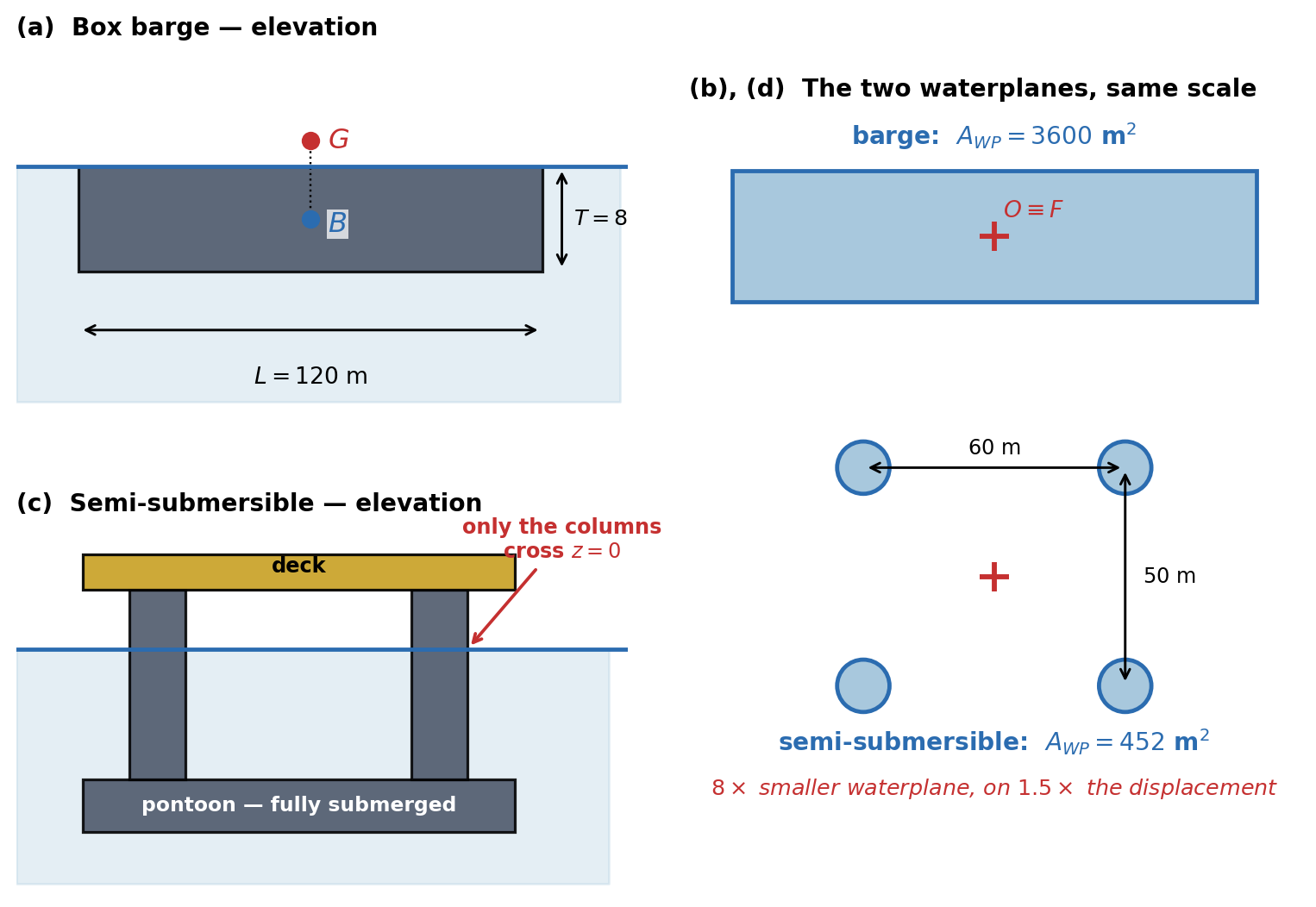
The first is a rectangular box barge, \(L = 120\) m, \(B = 30\) m, floating at an even-keel draft \(T = 8\) m with its centre of gravity \(KG = 10\) m above the keel. Its waterplane is a full rectangle, so every integral in \(\boldsymbol{C}\) can be done in closed form and checked by hand — which is exactly why it is used here.
The second is a semi-submersible drilling unit of \(45\,000\) t displacement, floating on four circular columns of \(12\) m diameter whose centres sit at \(x = \pm 30\) m and \(y = \pm 25\) m, with the bulk of the buoyancy in submerged pontoons well below the surface. Its waterplane is four small circles and nothing else.
Both float. They respond to the sea in completely different ways, and the whole of that difference is written in \(A_{WP}\).
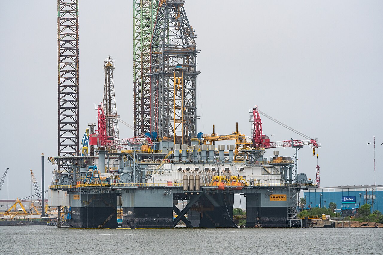
Figure 6.6 sets the two hulls side by side. The elevations show where the buoyancy is; the waterplanes, drawn to a common scale, show where the stiffness comes from — and they are what Problems 1–4 are really about.
The stiffness matrix of a box barge. Take the barge described above, with the BCS origin at midship on the waterline.
- Evaluate \(A_{WP}\), \(\nabla\), the displacement mass \(m\), and the waterplane integrals \(I_x^A\), \(I_y^A\), \(I_{xy}^A\), \(I_{xx}^A\) and \(I_{yy}^A\) about the BCS origin. State which of them vanish and give the geometric reason in each case.
- Obtain \(KB\), \(BM_T\), \(BM_L\) and hence \(GM_T\) and \(GM_L\). Assemble the full \(6\times6\) matrix \(\boldsymbol{C}\).
- \(\boldsymbol{C}\) has three zero rows and three zero columns. Name the degrees of freedom they belong to and explain, from the physical argument of this chapter rather than from the algebra, why a freely floating body has no hydrostatic stiffness in them at all. What consequence does this have for a vessel that must hold station?
- The ratio \(GM_L/GM_T\) for this barge is large. Compute it, and explain which single geometric quantity is responsible for essentially all of it.
- Taking the radii of gyration about \(G\) as \(k_x = 0.35B\) and \(k_y = 0.25L\), and ignoring added mass entirely, estimate the natural periods in heave, roll and pitch. Which of the three will be most in error when added mass is put back, and why?
Moving the origin creates coupling that was never there. The barge of Problem 1 is unchanged in every physical respect, but a designer chooses to place the BCS origin at a convenient structural frame \(12\) m aft of midship instead of at midship. The hull, its draft and its loading are all exactly as before.
- In the new BCS the waterplane still spans the same rectangle, but is no longer centred on the origin. Evaluate \(I_x^A\) and \(I_{xx}^A\) about the new origin, and hence write down the new \(GM_L\) and the new \(\boldsymbol{C}\).
- The matrix now has non-zero entries \(C_{35} = C_{53}\). Give the physical statement each of these two entries makes — one sentence for \(C_{35}\) read as “a pitch produces a heave force”, and one for \(C_{53}\) read as “a heave produces a pitch moment”.
- Express the coupling as the dimensionless ratio \(|C_{35}|/\sqrt{C_{33}C_{55}}\). Is the coupling weak or strong?
- \(GM_L\) came out larger than in Problem 1. A student concludes that the barge has become more stable in pitch simply because the origin was moved. Identify the error, and state what physical quantity has genuinely not changed. Demonstrate it: take the radii of gyration of Problem 1(e), place \(G\) on the same vertical as the midship waterplane centroid at \(KG = 10\) m, and solve the coupled heave–pitch eigenvalue problem \(\det(-\omega^2\boldsymbol{M} + \boldsymbol{C}) = 0\) in both coordinate choices.
- State the one condition on the choice of origin that makes \(C_{35}\) vanish, and explain why designers nevertheless often accept a non-zero \(C_{35}\).
A tank of ballast water that is not where you think it is. The barge of Problem 1 (origin back at midship) is fitted with a rectangular ballast tank \(20\) m long and \(15\) m wide, partially filled with sea water. The tank is deep enough that its free surface stays clear of the top and bottom at all angles considered. The total mass of the barge and its contents, and the position of \(G\), are exactly as in Problem 1 — the ballast has already been counted in both.
- When the barge rolls by a small angle, the water in the tank runs to the low side. Explain, using the same two-part argument this chapter uses for the hull itself (\(G\)–\(B\) separation plus a waterplane integral), why this produces a moment that reduces the restoring moment rather than adding to it.
- The loss of transverse metacentric height caused by a free liquid surface is \(\delta GM_T = i_t/\nabla\), where \(i_t\) is the second moment of the tank’s free surface area about its own centreline. Evaluate \(\delta GM_T\) and the corrected \(GM_T\) and \(C_{44}\).
- Compute the roll natural period before and after, using \(k_x = 0.35B\) and a roll added inertia of \(0.20\,I_{44}\). By what percentage does the period change, and in which direction?
- Suppose the tank is \(6\) m deep and half full, so it holds roughly \(3\%\) of the barge’s displacement. Show, from the form of \(i_t\), why the amount of water is not what governs the loss at all, and state the single tank dimension a designer should attack first. Quantify the benefit of splitting the tank in two with a centreline bulkhead.
- Does \(\delta GM_T\) depend on how much water is in the tank? Does it depend on the density of the liquid in it? Answer both, and identify the practical measure used aboard ship to control this effect.
Why a drilling rig is built on four thin legs. Take the semi-submersible described above: displacement \(45\,000\) t, four circular columns of diameter \(D = 12\) m piercing the free surface with centres at \(x = \pm 30\) m, \(y = \pm 25\) m, and all remaining buoyancy in fully submerged pontoons. The heave added mass is large for such a form; take \(A_{33} = 1.5\,m\).
- Evaluate \(A_{WP}\) and \(C_{33}\), and compare \(A_{WP}\) with that of the barge of Problem 1. Explain why the submerged pontoons, which carry most of the buoyancy, contribute nothing to \(A_{WP}\).
- Compute the heave natural period, first ignoring added mass and then with \(A_{33} = 1.5\,m\). Do the same for the barge of Problem 1, using \(A_{33} = 1.0\,m\) there.
- Ocean waves that carry significant energy have periods roughly in the band \(5\)–\(20\) s. Place all four heave periods from part (b) on that band and state, in one sentence for each vessel, what the design achieves.
- Evaluate \(I_{xx}^A\) and \(I_{yy}^A\) for the four-column waterplane, treating each column both as a point area at its centre and with its own \(\pi D^4/64\), and comment on the size of the self term. Hence obtain \(BM_T\) and \(BM_L\).
- The rig’s designers made \(A_{WP}\) as small as they dared, but not smaller. Give the two distinct penalties of shrinking the columns further — one that appears in \(\boldsymbol{C}\), and one that concerns what happens when a load is added to the deck.
Throwing away viscosity, and knowing when you may not. This chapter justifies an inviscid fluid by the estimate \(F_v/F_p \sim \nu^{1/2}\omega^{3/2}/g\), obtained with a boundary layer thickness \(\delta \sim \sqrt{\nu/\omega}\).
- A \(200\) m ship radiates waves of its own length in deep water. Using the deep water dispersion relation \(\omega = \sqrt{gk}\) with \(k = 2\pi/\lambda\) and \(\lambda = L\), find \(\omega\), then \(\delta\) and the ratio \(F_v/F_p\). Repeat for a \(2\) m model of the same hull tested at the same \(\lambda/L\).
- The ratio grows as \(\omega^{3/2}\), and the model runs at a higher frequency. By what factor does \(F_v/F_p\) increase from ship to model? Is the inviscid assumption still safe for the model?
- Evaluate \(\delta\) for both. Compare each with its hull length and comment on the picture of the flow this justifies.
- Radiation damping and viscous damping are physically unrelated, yet both remove energy from a rolling ship. For the \(200\) m ship in roll, state which of the two dominates and why the argument of parts (a)–(c) does not settle the question. Name the geometric feature commonly fitted to exploit this.
- A colleague proposes to check a potential flow code by setting \(\nu = 0\) in a viscous CFD solver and expecting the radiation damping \(B_{33}\) to fall to zero. Explain what would actually happen and why.
What linearization actually costs. This problem is about the boundary value problem summarised in the interactive anatomy of the boundary value problem, and needs no arithmetic beyond part (d).
- Of the six statements that make up the problem — Laplace’s equation, the kinematic and dynamic free surface conditions, the bottom condition, the radiation condition and the body condition — state which are exactly linear before any approximation is made, and which are not. For each nonlinear one, point to the specific term responsible.
- A student says “we linearize the governing equation to make the problem solvable.” Correct the statement precisely, and say where all of the approximation in this chapter actually lives.
- Linearization does two distinct things to the free surface condition. One is dropping terms; the other is a change of where the condition is imposed. State both, and explain why the second is what makes the problem solvable at all, given that the free surface elevation is itself an unknown.
- A barge of \(8\) m draft oscillates in heave with amplitude \(0.4\) m in waves of \(2\) m amplitude and \(80\) m length. Estimate the wave slope \(\epsilon = ka\) and the ratio (motion amplitude)/(draft). On this evidence, is first order theory reasonable? Now repeat for a storm with \(8\) m amplitude waves of the same length and a \(2.0\) m heave, and comment.
- Once linearized, the problem is split into six sub-problems, one per degree of freedom, each solved one frequency at a time. Name the two distinct principles that license these two splittings, and state what would be lost if either failed.
Problems 7–10 leave hydrostatics behind and deal with the radiation problem. Figure 6.7 shows the two things they turn on: where radiation damping physically comes from, and why the natural frequency of Problem 7 is a fixed point rather than a formula.
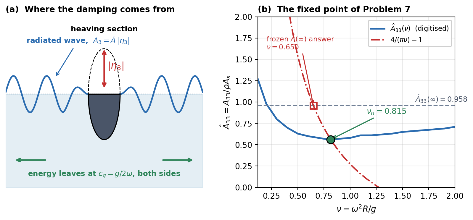
A natural frequency you cannot solve for in one step. A long horizontal circular cylinder of radius \(R = 10\) m floats with its axis in the calm free surface and heaves in deep water. All quantities are per unit length: the mass is \(m' = \rho A_s\) with \(A_s = \tfrac12\pi R^2\), and the heave stiffness is \(K' = \rho g (2R)\), the waterplane breadth being the diameter. This is the section of the radiation simulation above. Its non-dimensional added mass \(\hat{A}_{33} = A_{33}/(\rho A_s)\), digitised from Fig. 3.6 of Faltinsen (1990) as a function of \(\nu = \omega^2R/g\), is the data plotted by that simulator:
\(\nu\) 0.4 0.5 0.6 0.7 0.8 0.9 1.0 1.2 \(\hat{A}_{33}\) 0.700 0.630 0.600 0.580 0.560 0.570 0.580 0.610 Interpolate linearly between the tabulated points. The infinite frequency value is \(\hat{A}_{33}(\infty) = 0.958\).
- Verify that \(m'\) and \(K'\) give \(\omega_n^2 = K'/(m' + A_{33})\), and show that in non-dimensional form the condition becomes \(\nu\left(1 + \hat{A}_{33}(\nu)\right) = 4/\pi\), independent of \(R\). Explain what that independence means physically.
- Solve the fixed point iteration \(\nu_{i+1} = (4/\pi)/(1 + \hat{A}_{33}(\nu_i))\) starting from \(\nu_0 = 0.8\). Tabulate the first five iterates and give the converged \(\nu_n\), \(\omega_n\) and \(T_n\).
- Now do it the naive way: freeze the added mass at its infinite frequency value \(\hat{A}_{33}(\infty) = 0.958\) and solve in one step. Report the resulting \(T_n\) and the percentage error against part (b).
- Repeat parts (b) and (c) for \(R = 4\) m and \(R = 16\) m. Confirm that the percentage error is the same at all three radii, and explain why that had to be so.
- A designer asks why \(\boldsymbol{A}(\omega)\) cannot simply be replaced by a single constant “entrained mass of water”, as an undergraduate textbook suggests. Answer using your numbers, and state the one circumstance in which a constant added mass is legitimate.
Damping without friction. The same cylinder, \(R = 10\) m, now heaves at \(\omega = 0.94\) rad/s with amplitude \(|\eta_3| = 1.5\) m in deep water. At this frequency \(\nu = \omega^2R/g \simeq 0.90\), a tabulated point of the digitised data of Faltinsen (1990), where \(\hat{B}_{33} = 0.420\), where \(B_{33} = \hat{B}_{33}\,\rho\,\omega A_s\) and \(A_s = \tfrac12\pi R^2\). The fluid is inviscid throughout.
- Evaluate \(\nu\), \(B_{33}\), and the radiated wave amplitude ratio \(\bar{A} = A_3/|\eta_3|\) from the energy relation \(\eqref{eq-faltinsen-326}\), \(\bar{A} = \nu\sqrt{\pi\hat{B}_{33}/2}\). What is the height of the radiated wave?
- Compute the average power dissipated per unit length, \(\bar{P} = \tfrac12 B_{33}\omega^2|\eta_3|^2\), and the energy removed per cycle.
- Verify that answer independently: a deep water wave of amplitude \(A_3\) carries mean energy \(\tfrac12\rho g A_3^2\) per unit area, transported at the group velocity \(c_g = g/2\omega\). Two wave trains leave the cylinder, one to each side. Show that the power they carry equals \(\bar{P}\), and state what this identity proves about the origin of \(B_{33}\).
- The energy is leaving the body. Where does it go, and in what sense is it “lost”? Contrast this carefully with the dashpot of Chapter 2.
- From \(\eqref{eq-faltinsen-326}\), argue that \(B_{33} \ge 0\) always, whereas \(A_{33}\) carries no such guarantee and is in fact negative for some sections. Why does the argument constrain one and not the other?
Why the time domain needs a convolution. A single degree of freedom (heave) model of a floating body has, per unit length, \(m + A_{33}(\infty) = 4.00\times10^{5}\) kg/m and \(C_{33} = 2.00\times10^{5}\) N/m per m. Its radiation damping is well represented over all frequencies by \[B_{33}(\omega) = B_0\frac{\omega^2}{\omega^2 + p^2}, \qquad B_0 = 2.00\times10^{5}\ \text{kg/(m·s)}, \quad p = 0.50\ \text{rad/s}\]
- State \(B_{33}(0)\) and \(B_{33}(\infty)\), and give the physical meaning of each limit for a heaving body.
- Using \(\boldsymbol{K}(\tau) = \frac{2}{\pi}\int_0^\infty\left(\boldsymbol{B}(\omega) - \boldsymbol{B}(\infty)\right)\cos(\omega\tau)\,d\omega\) and the standard integral \(\int_0^\infty \frac{\cos\omega\tau}{\omega^2+p^2}d\omega = \frac{\pi}{2p}e^{-p\tau}\), show that \(K(\tau) = -B_0\,p\,e^{-p\tau}\). Evaluate \(K(0)\) and the memory time over which \(K\) decays to \(1\%\) of that value.
- Recover \(A_{33}(\omega) - A_{33}(\infty)\) from \(K(\tau)\) using \(A(\omega) = A(\infty) - \frac{1}{\omega}\int_0^\infty K(\tau)\sin(\omega\tau)d\tau\), and evaluate it at \(\omega = 0.3\), \(0.8\) and \(1.5\) rad/s. Confirm your result numerically.
- Write out the Cummins equation for this body in free decay, and explain in one sentence what the convolution term is physically doing that \(\boldsymbol{B}(\infty)\{\dot\xi\}\) alone cannot.
- A student proposes to skip the convolution and simply use \(-A_{33}(\omega_n)\ddot\xi - B_{33}(\omega_n)\dot\xi\) with the coefficients evaluated once at the natural frequency. State the one situation in which this is exactly right, and one realistic situation in which it fails badly.
Programming Problem: A heave decay test in the time domain. Simulate the free decay of the body of Problem 9, released from rest at \(\xi_3(0) = 1.0\) m with \(\dot\xi_3(0) = 0\) and no motion before \(t = 0\). Because \(K(\tau) = -B_0pe^{-p\tau}\) is a single decaying exponential, the convolution can be replaced exactly by one extra state variable: define \[\mu(t) = \int_{-\infty}^{t}K(t-\tau)\dot\xi_3(\tau)\,d\tau \qquad\Longrightarrow\qquad \dot\mu = -p\,\mu + K(0)\,\dot\xi_3\]
- Verify that state space form of the convolution by differentiating the integral, and write the three first-order equations to be integrated.
- Integrate to \(t = 60\) s and report the first four peak times. Estimate the damped period and the logarithmic decrement from the peaks, and say why the very first interval — from the release at \(t=0\) to the first peak — should be excluded from that estimate.
- Because the memory state \(\mu\) is a third state variable, this system is third order, not second, and its damped period can be obtained exactly from the roots of the characteristic cubic. Derive that cubic, find its roots, and compare the exact damped period with three estimates: the simulation of part (b), the frequency domain fixed point \(-\omega^2\left(m + A_{33}(\omega)\right) + C_{33} = 0\) using \(A_{33}(\omega)\) from Problem 9(c), and the crude \(A_{33}(\infty)\) value. Rank them, and say what the residual error of the fixed point estimate is telling you.
- Re-run with the convolution deleted (that is, with \(\mu \equiv 0\), keeping \(B_{33}(\infty)\)). Report the period and the decrement, and explain the direction of both errors.
- The retardation function here is negative for all \(\tau\). Explain what that means for the sign of the memory force during a decay, and reconcile it with the requirement that the total damping still removes energy.
Answer Key
Problem 1 — The stiffness matrix of a box barge
- (a) \(A_{WP} = LB = 3600\) m\(^2\), \(\nabla = LBT = 28800\) m\(^3\), and \(m = \rho\nabla = 2.9520 \times 10^{7}\) kg (\(29.52\times10^{3}\) t). For the second moments, \(I_{xx}^A = BL^3/12 = 4.3200 \times 10^{6}\) m\(^4\) and \(I_{yy}^A = LB^3/12 = 2.7000 \times 10^{5}\) m\(^4\). The three that vanish are \(I_x^A = \iint x\,dA = 0\) and \(I_y^A = \iint y\,dA = 0\), because the origin is at the waterplane centroid (the centre of flotation \(F\)), so the first moments about it are zero by definition of a centroid; and \(I_{xy}^A = \iint xy\,dA = 0\), because the waterplane is symmetric about \(y=0\), so every element at \(+y\) is matched by an identical one at \(-y\) and the products cancel in pairs.
- (b) \(KB = T/2 = 4.00\) m for a box. \(BM_T = I_{yy}^A/\nabla = 9.3750\) m and \(BM_L = I_{xx}^A/\nabla = 150.00\) m. Hence \(GM_T = KB + BM_T - KG = 4.00 + 9.3750 - 10.00 = 3.3750\) m and \(GM_L = 144.00\) m. The matrix is \[\boldsymbol{C} = \begin{bmatrix} 0 & 0 & 0 & 0 & 0 & 0 \\ 0 & 0 & 0 & 0 & 0 & 0 \\ 0 & 0 & 3.620\!\times\!10^{7} & 0 & 0 & 0 \\ 0 & 0 & 0 & 9.774\!\times\!10^{8} & 0 & 0 \\ 0 & 0 & 0 & 0 & 4.170\!\times\!10^{10} & 0 \\ 0 & 0 & 0 & 0 & 0 & 0 \end{bmatrix} \] in N/m, N and N·m as appropriate, with the only non-zero entries at \((3,3)\), \((4,4)\) and \((5,5)\) — heave, roll and pitch are uncoupled here precisely because the two first moments \(I_x^A\), \(I_y^A\) and the product moment \(I_{xy}^A\) all vanished in part (a).
- (c) Surge, sway and yaw. Each of them moves the hull in the horizontal plane only, so the instantaneous underwater volume is unchanged, the buoyancy force is unchanged in both magnitude and line of action, and \(G\) and \(B\) stay in the same vertical line. With nothing changed, there is nothing to restore: the water does not know the barge has moved. The consequence is that a freely floating body is neutrally stable in these three modes — it will drift and yaw indefinitely under any residual force. Station keeping in surge, sway and yaw therefore has to be supplied, by mooring lines or by thrusters under dynamic positioning; there is no hydrostatic help available, which is why those systems exist at all.
- (d) \(GM_L/GM_T = 42.7\). The two metacentric heights differ only through \(BM = I^A/\nabla\), since both carry the same \(KB - KG = -6.00\) m. Because \(I_{xx}^A = BL^3/12\) while \(I_{yy}^A = LB^3/12\), the two radii are in the ratio \(BM_L/BM_T = (L/B)^2 = 16\): the length-to-beam ratio, entering cubed in the waterplane integral, is what creates the disparity. The final ratio of \(GM\)s is larger still, \(42.7\) rather than \(16\), because the common negative term \(KB - KG\) subtracts the same \(6.00\) m from both and so eats a large fraction of the small transverse value while barely touching the longitudinal one. This is why a ship is enormously stiffer in pitch than in roll, and why roll, not pitch, is the mode that gives trouble at sea.
- (e) With \(k_x = 10.50\) m and \(k_y = 30.00\) m, \(I_{44} = 3.2546 \times 10^{9}\) and \(I_{55} = 2.6568 \times 10^{10}\) kg·m\(^2\). Then \(T_3 = 2\pi\sqrt{m/C_{33}} = 5.67\) s, \(T_4 = 2\pi\sqrt{I_{44}/C_{44}} = 11.47\) s and \(T_5 = 5.02\) s. Heave will be most in error. The heave added mass of a beamy flat-bottomed hull is comparable with the displacement itself, \(A_{33} \sim m\), so \(T_3\) can be out by \(30\)–\(40\%\); the roll and pitch added inertias are typically only \(10\)–\(20\%\) of the corresponding rigid body values, because rotating the hull sets far less water in motion than heaving it bodily. Problem 5 puts the numbers to this.
Problem 2 — Moving the origin creates coupling that was never there
- (a) The centroid of the waterplane now lies at \(x_F = +12\) m in the new BCS, so \(I_x^A = \iint x\,dA = A_{WP}x_F = 4.3200 \times 10^{4}\) m\(^3\), no longer zero. By the parallel axes theorem for areas, \(I_{xx}^A = BL^3/12 + A_{WP}x_F^2 = 4.8384 \times 10^{6}\) m\(^4\), giving \(BM_L = 168.00\) m and \(GM_L = 162.00\) m. The matrix gains one symmetric off-diagonal pair, \(C_{35} = C_{53} = -\rho g I_x^A = -4.3439 \times 10^{8}\) N: \[\boldsymbol{C} = \begin{bmatrix} 0 & 0 & 0 & 0 & 0 & 0 \\ 0 & 0 & 0 & 0 & 0 & 0 \\ 0 & 0 & 3.620\!\times\!10^{7} & 0 & -4.344\!\times\!10^{8} & 0 \\ 0 & 0 & 0 & 9.774\!\times\!10^{8} & 0 & 0 \\ 0 & 0 & -4.344\!\times\!10^{8} & 0 & 4.691\!\times\!10^{10} & 0 \\ 0 & 0 & 0 & 0 & 0 & 0 \end{bmatrix}\]
- (b) First fix the sign convention. With \(x\) towards the bow and \(z\) up, a positive pitch \(\xi_5\) is a rotation that carries the bow downwards and the stern up: the local change of draft at station \(x\) is \(x\,\xi_5\), which is an increase in immersion for \(x>0\). (This is the same convention as \(\Delta\nabla = \iint_{A_{WP}} x\,\xi_5\,dA\) in the text.) \(C_{35}\) — a pitch produces a heave force: the pitch immerses everything forward of the origin and lifts everything aft of it. Were the origin at the centre of flotation the two wedges would cancel exactly and there would be no net change of displaced volume; but the origin now sits \(12\) m aft of \(F\), so the immersing part of the waterplane is the larger one, the gain forward outweighs the loss aft, and the body acquires extra buoyancy — a net upward force, even though it has not heaved. Consistently, \(\tau_{hst,3} = -C_{35}\xi_5 = +\rho g I_x^A \xi_5 > 0\). \(C_{53}\) — a heave produces a pitch moment: a downward heave (\(\xi_3 < 0\)) immerses the whole waterplane uniformly and generates extra buoyancy, and that extra force acts through the centre of flotation \(F\), the centroid of the added layer. \(F\) is \(12\) m forward of the origin about which moments are taken, so an upward force on a \(12\) m lever is a bow-up, i.e. negative, pitch moment — again \(\tau_{hst,5} = -C_{53}\xi_3 = \rho g I_x^A \xi_3 < 0\) — even though the body has not pitched. The two coefficients are equal because both are the same integral \(\rho g \iint x\,dA\); the symmetry of \(\boldsymbol{C}\) is not a coincidence but a statement that the restoring forces derive from a potential energy.
- (c) \(|C_{35}|/\sqrt{C_{33}C_{55}} = 0.3333\), i.e. about \(33\%\). This is strong coupling — not a rounding effect. A heave decay test on this barge, analysed as though heave were an independent single degree of freedom system, would be contaminated by a visible pitch oscillation.
- (d) The error is treating \(GM_L\) as a property of the vessel when it is a property of the vessel together with the point moments are taken about. Nothing physical has changed: the hull, the displacement, the loading and the water are identical, and the barge is neither more nor less stable than before. The larger \(GM_L\) is exactly offset by the new \(C_{35}\) coupling and by the matching change in the mass matrix, which acquires its own \(-m x_G\) terms about the shifted origin. What is genuinely invariant are the natural frequencies of the coupled system. Solving \(\det(-\omega^2\boldsymbol{M}+\boldsymbol{C}) = 0\) in the heave–pitch plane for both choices gives \[\omega_n = (1.107362,\ 1.250062) \text{ rad/s at midship}, \qquad \omega_n = (1.107362,\ 1.250062) \text{ rad/s at the shifted origin}\] identical to every digit shown (periods \(5.6740\) s and \(5.0263\) s), even though \(GM_L\), \(C_{55}\) and \(C_{35}\) all differ between the two. This is the decisive test of any hydrostatics implementation: change the origin, and the predicted periods must not move.
- (e) \(C_{35} = -\rho g\iint x\,dA\) vanishes if and only if the origin is placed so that \(x_F = 0\) — that is, on the same longitudinal station as the centre of flotation, the centroid of the waterplane. Designers frequently do not, for the same reason met in Chapter 5 for the centre of gravity: \(F\) is not a fixed point of the structure. It migrates as the vessel changes draft and trim, so an origin locked to \(F\) would move with every loading condition and make all hull geometry, sensor positions and mass properties condition dependent. A fixed structural origin buys constant geometry at the price of the off-diagonal terms — and since \(\boldsymbol{C}\) is assembled numerically anyway, that price is nearly zero.
Problem 3 — A tank of ballast water that is not where you think it is
- (a) The two effects are exactly those of the hull, but applied to the tank and with the signs reversed. First, the tank’s own waterplane tips with the barge, so a wedge of water is transferred from the high side to the low side: this shifts the centre of gravity of the liquid — and hence of the whole vessel — towards the low side, in the same direction as the heel. Whereas the hull’s transferred wedge moves the centre of buoyancy to the low side and so creates a righting couple, the tank’s transferred wedge moves the centre of gravity to the low side and so creates a heeling couple, directly opposing it. Second, the \(G\)–\(B\) part of the argument still applies, but with \(G\) now displaced horizontally by the shift, the lever between weight and buoyancy is reduced by exactly that amount. Both effects say the same thing: the moment is proportional to the tank’s own waterplane integral \(\iint_{A_t} y^2\,dA = i_t\), it acts against the restoring moment, and it is therefore subtracted.
- (b) \(i_t = l_t b_t^3/12 = 20\times15^3/12 = 5625.0\) m\(^4\), so \(\delta GM_T = i_t/\nabla = 5625.0/28800 = 0.1953\) m. The corrected value is \(GM_T = 3.3750 - 0.1953 = 3.1797\) m, a loss of \(5.8\%\) of the stability margin. Correspondingly \(C_{44}\) falls from \(9.7737 \times 10^{8}\) to \(9.2081 \times 10^{8}\) N·m/rad.
- (c) With \(k_x = 10.50\) m the rigid body roll inertia is \(3.2546 \times 10^{9}\) kg·m\(^2\); including the \(20\%\) added inertia, \(I_{44} + A_{44} = 3.9055 \times 10^{9}\) kg·m\(^2\). Then \(T_4 = 12.560\) s before and \(12.940\) s after — an increase of \(3.03\%\). The period lengthens, because the free surface has removed stiffness while leaving the inertia untouched, and \(T \propto 1/\sqrt{C_{44}}\). A lengthening roll period measured at sea is in fact one of the classical warning signs that a vessel has lost stability.
- (d) \(\delta GM_T = i_t/\nabla = l_t b_t^3/(12\nabla)\) contains no mass and no density of the tank contents at all — only the geometry of the free surface. The effect is not caused by the weight of the water but by its freedom to move, so a shallow puddle spread over a wide tank is as damaging as a deep one. Since \(i_t \propto b_t^3\), the tank’s breadth is the dimension to attack. Fitting a centreline bulkhead leaves the same total tank area, the same volume and the same mass of ballast, but replaces one surface of breadth \(b_t\) by two of breadth \(b_t/2\): \(i_t \rightarrow 2\,l_t(b_t/2)^3/12 = 1406.2\) m\(^4\), exactly \(1/4\) of \(5625.0\) m\(^4\), so \(\delta GM_T\) falls from \(0.1953\) m to \(0.0488\) m. The cube on \(b_t\) is doing all the work: longitudinal subdivision buys three quarters of the loss back for the price of one bulkhead, and this, not the weight of the ballast, is why tanks are built long and narrow rather than short and wide.
- (e) No to how much: the formula involves only the area of the free surface and its second moment, so a tank one tenth full and one tenth from full give the same \(\delta GM_T\), provided the surface still spans the full breadth of the tank. It vanishes only in the two limits where there is no free surface at all — completely empty or pressed full. Yes to the density, in general: the exact loss is \(\rho_t i_t/(\rho\nabla)\), so a tank of fuel oil (\(\rho_t \approx 0.85\rho\)) is about \(15\%\) less damaging than one of sea water; the form quoted in part (b) assumes the tank holds the same sea water as the vessel floats in. The practical measures are exactly those two limits: tanks are kept either pressed full or empty, slack tanks are minimised in number, and where a tank must be slack it is subdivided longitudinally as in part (d).
Problem 4 — Why a drilling rig is built on four thin legs
- (a) Each column cuts the free surface in a circle of area \(\pi D^2/4 = 113.10\) m\(^2\), so \(A_{WP} = 4\times113.10 = 452.4\) m\(^2\) and \(C_{33} = \rho g A_{WP} = 4.5489 \times 10^{6}\) N/m. The barge has \(A_{WP} = 3600\) m\(^2\), 8.0 times larger, on a displacement only \(0.66\) times as big. The pontoons contribute nothing because \(A_{WP}\) is the area of the body’s intersection with the plane \(z=0\), and the pontoons do not reach that plane. Heave stiffness is generated only by the change in displaced volume, \(\Delta\nabla \approx -A_{WP}\xi_3\), and moving a fully submerged body up or down by a small amount changes the volume it displaces not at all — it is submerged before and after. Buoyancy is supplied by volume; stiffness is supplied by waterplane area, and the semi-submersible deliberately separates the two.
- (b) Semi-submersible: ignoring added mass, \(T_3 = 2\pi\sqrt{m/C_{33}} = 19.8\) s; with \(A_{33} = 1.5m\) the inertia is \(2.5m\) and \(T_3 = 31.2\) s. Barge: \(5.67\) s without added mass and \(8.02\) s with \(A_{33} = m\). Added mass lengthens the period by \(58\%\) for the rig and \(41\%\) for the barge; in neither case is it a small correction, which is the practical reason \(\boldsymbol{A}(\omega)\) has to be computed rather than guessed.
- (c) The barge sits at \(8.0\) s, inside the \(5\)–\(20\) s band and in fact near the most energetic part of it: it is resonant with ordinary sea waves and will follow them, heaving with amplitudes comparable to the wave amplitude or worse. The rig sits at \(31\) s, well above the band. The barge is designed to float and be towed; the semi-submersible is designed to hold a drill string steady, and it achieves that by placing its heave natural period beyond the reach of any wave that carries appreciable energy, so that it is stiff to the sea in the only sense that matters — it is excited far above resonance and therefore barely responds. This is the same off-resonance strategy met in Chapter 2, applied by choosing \(A_{WP}\).
- (d) The point-area (parallel axes) terms are \(\sum A_c x_i^2 = 4.0715 \times 10^{5}\) m\(^4\) and \(\sum A_c y_i^2 = 2.8274 \times 10^{5}\) m\(^4\), while the self term is \(4\times\pi D^4/64 = 4071.5\) m\(^4\) for both. The self term is only \(0.99\%\) of \(I_{xx}^A\) and \(1.42\%\) of \(I_{yy}^A\) — negligible, because the columns are far apart compared with their own size (\(x_i/D = 2.5\)), and the separation enters squared. Hence \(I_{xx}^A = 4.1122 \times 10^{5}\) m\(^4\), \(I_{yy}^A = 2.8681 \times 10^{5}\) m\(^4\), and with \(\nabla = m/\rho = 43902\) m\(^3\), \(BM_L = 9.37\) m and \(BM_T = 6.53\) m. Note how modest these are next to the barge’s \(BM_L = 150\) m: the rig buys its angular stability almost entirely from the spacing of the columns, which is why the deck is so much wider than the structure needs to be for strength alone.
- (e) First, in \(\boldsymbol{C}\): every entry of the restoring matrix that is not zero is proportional to a waterplane integral — \(C_{33}\) to \(A_{WP}\), and \(C_{44}\), \(C_{55}\) to \(\nabla BM = \rho g I^A\), itself proportional to column area. Shrinking the columns therefore weakens roll and pitch stiffness at the same time as heave, and the rig eventually loses the angular stability it needs to keep the deck level and the drill string vertical. Second, and usually binding first: with \(C_{33} = \rho g A_{WP}\) very small, the change in draft caused by adding a deck load is \(\delta T = W/(\rho g A_{WP})\), which is inversely proportional to \(A_{WP}\). For this rig a \(1000\) t load sinks it by \(2.16\) m, against only \(0.271\) m for the barge — a factor of 8. A rig with columns half as thick would sink four times as far again for the same load, so its variable deck load, freeboard and air gap under the deck would all become unmanageable. The column diameter is a compromise between wanting a soft rig in waves and needing a rig whose draft does not change every time something is craned aboard.
Problem 5 — Throwing away viscosity, and knowing when you may not
- (a) Ship: \(k = 2\pi/200 = 0.03142\) m\(^{-1}\), \(\omega = \sqrt{gk} = 0.5551\) rad/s (period \(11.3\) s). \(\delta = \sqrt{\nu/\omega} = 1.3421\) mm and \(F_v/F_p \sim \nu^{1/2}\omega^{3/2}/g = 4.22 \times 10^{-5}\). Model: \(\omega = 5.5515\) rad/s (period \(1.13\) s), \(\delta = 0.4244\) mm, \(F_v/F_p = 1.33 \times 10^{-3}\).
- (b) The frequency ratio is \(\omega_m/\omega_s = \sqrt{L_s/L_m} = 10.0\), so the force ratio grows by \((\omega_m/\omega_s)^{3/2} = 31.6\), from \(4.22 \times 10^{-5}\) to \(1.33 \times 10^{-3}\). Yes, still safe — even at \(1.33 \times 10^{-3}\) the viscous contribution to the radiation problem is around about one part in a thousand, still far below the accuracy of any measurement. But notice the direction of the trend: it is the model, not the ship, that is relatively more viscous. Scale effects in a towing tank always run this way, which is why model tests are corrected for viscosity before being scaled up, and never the reverse.
- (c) \(\delta/L = 6.71 \times 10^{-6}\) for the ship and \(2.12 \times 10^{-4}\) for the model. In absolute terms \(\delta\) is about a millimetre for the ship (\(1.34\) mm, roughly the thickness of a small coin) and under half a millimetre for the model (\(0.42\) mm) — a skin some \(1.5\times10^{5}\) times thinner than the ship it clings to, and \(4.7\times10^{3}\) times thinner than the model. This is exactly the picture that justifies potential flow: vorticity generated at the hull is confined to a skin so thin that, as far as the pressure field and the radiated waves are concerned, the fluid may be treated as irrotational right up to the hull, and the no-slip condition may be replaced by the far weaker requirement that fluid merely not pass through the surface.
- (d) In roll, viscous damping usually dominates, and often by a large margin — the opposite of the conclusion for heave. The estimate of part (a) does not settle the question because it compares the viscous force with the pressure force, and finds it negligible; but the quantity that matters for decay is the small damping part of the pressure force. For a roll motion the hull is nearly wall-sided and rotating about an axis near the waterline, so it is extremely inefficient at radiating waves: \(B_{44}\) from potential theory is very small, and a viscous effect that is negligible against \(F_p\) need not be negligible against that particular small piece of it. Worse, the dominant viscous roll damping is not the thin-boundary-layer skin friction assumed in the scaling at all, but flow separation and eddy shedding at the bilges, which the \(\delta \sim \sqrt{\nu/\omega}\) picture does not describe. The feature fitted to exploit this is the bilge keel — a long fin along the turn of the bilge whose only purpose is to force separation and shed vortices, and which can easily double or triple the total roll damping. This is why roll is the one degree of freedom for which a purely potential flow prediction is never trusted, and why empirical or model-test damping is added by hand.
- (e) \(B_{33}\) would not fall to zero; it would barely change. The radiation damping of this chapter is not friction, and contains no viscosity: it is the rate at which energy is carried away from the body by the radiated waves, which propagate off to infinity and never return, as the exact energy statement \(\eqref{eq-faltinsen-326}\) makes explicit — \(B_{33}\) is fixed by the amplitude of the wave the body makes. An inviscid solver still radiates waves; setting \(\nu = 0\) removes the boundary layer, not the free surface. The colleague’s test would only confirm what the chapter already argues: the fluid is assumed inviscid throughout, and \(\boldsymbol{B}(\omega)\) is computed from \(\hat\varphi_k^{(1)}\) with viscosity nowhere in the formulation. The one way to make \(B_{33}\) vanish is to remove the free surface — oscillate the same body deep underwater, where it radiates nothing and the damping genuinely is zero while the added mass survives.
Problem 6 — What linearization actually costs
- (a) Exactly linear already: Laplace’s equation \(\nabla^2\varphi = 0\); the bottom condition \(\partial\varphi/\partial z = 0\) on \(z = -h\); and the radiation condition at \(S_\infty\). Nonlinear: the two free surface conditions and the body condition. In the kinematic free surface condition the offending terms are the products of unknowns \(\frac{\partial\varphi}{\partial x}\frac{\partial\eta}{\partial x} + \frac{\partial\varphi}{\partial y}\frac{\partial\eta}{\partial y}\), and, just as importantly, the fact that it is imposed on \(z = \eta(x,y,t)\) — an unknown surface. In the dynamic condition the offender is the quadratic \(\tfrac{1}{2}|\nabla\varphi|^2\), again on the unknown \(z = \eta\). In the body condition the nonlinearity is that it is applied on \(S_B(t)\), the instantaneous wetted surface, whose position depends on the motion \(\{\xi\}\) that we are trying to find — the condition and the unknown are entangled.
- (b) The statement is wrong in its premise. Laplace’s equation is already linear and is never linearized — it is not the difficulty. Every order of the perturbation series satisfies the identical governing equation \(\nabla^2\varphi^{(n)} = 0\). All of the approximation in this chapter lives entirely in the boundary conditions: the two free surface conditions and the body condition. A useful way to hold this: the physics of the interior of the fluid is easy and exact; the difficulty is the shape of the region and what happens on its edges.
- (c) (i) Terms are dropped: the quadratic products \(\nabla\varphi\cdot\nabla\eta\) and \(\tfrac12|\nabla\varphi|^2\), being of order \(\epsilon^2\), are discarded, leaving conditions in which \(\varphi^{(1)}\) and \(\eta^{(1)}\) appear linearly. (ii) The condition is transferred, by Taylor expanding about \(z = 0\), from the unknown surface \(z = \eta\) to the known, fixed plane \(z = 0\) — and correspondingly the body condition is transferred from \(S_B(t)\) to the mean wetted surface \(S_{B0}\). The second is the decisive one. Before it, the problem is a free boundary problem: the domain in which the equation is to be solved is itself part of the answer, so one cannot even begin to discretise it. After it, the domain is fixed and known in advance, the boundaries can be meshed once, and the problem becomes an ordinary linear boundary value problem. Everything in this chapter — superposition into six modes, one frequency at a time, a constant panel mesh on \(S_{B0}\) — rests on the domain having stopped moving.
- (d) \(k = 2\pi/80 = 0.0785\) m\(^{-1}\). Moderate sea: \(\epsilon = ka = 0.157\) and \(\xi_3/T = 0.4/8 = 0.050\) — a wave slope of \(16\%\) and a motion of \(5\%\) of the draft. The neglected terms are of order \(\epsilon^2 \approx 0.025\) — roughly a \(2.5\%\) error. First order theory is entirely reasonable here. Storm: \(\epsilon = 0.628\) and \(\xi_3/T = 0.250\), so the neglected terms are of order \(0.39\), i.e. a \(39\%\) error — no longer a correction but a comparable quantity. Worse, the qualitative assumptions themselves fail: a wave of slope \(0.63\) is close to breaking, and a \(2\) m heave on an \(8\) m draft means the wetted surface differs from \(S_{B0}\) by a quarter of the draft, so transferring the body condition to \(S_{B0}\) is no longer defensible. Linear seakeeping is a fair weather theory; extreme response requires second order or fully nonlinear methods.
- (e) Superposition, and the Fourier decomposition of Chapter 3 — and both are available only because the linearized problem is linear in \(\varphi^{(1)}\) and its boundary data. Superposition licenses \(\varphi^{(1)} = \sum_{k=1}^{6}\tilde\varphi_k^{(1)}\): the potential due to six simultaneous motions is the sum of the potentials each would produce alone, so one intractable problem becomes six solvable ones. Fourier decomposition licenses solving one frequency at a time: an arbitrary small-amplitude motion is a sum of sinusoids, each of which can be treated independently and the responses added. If superposition failed, the six modes would interact and a rig heaving and pitching would need its own solution distinct from the sum of the two; if frequency separation failed, energy would pass between frequencies and \(\boldsymbol{A}(\omega)\), \(\boldsymbol{B}(\omega)\) — which are defined one frequency at a time — would not exist as functions of \(\omega\) at all. Both do in fact fail at second order, which is exactly where sum- and difference-frequency effects such as slow drift come from.
Problem 7 — A natural frequency you cannot solve for in one step
- (a) Undamped free heave gives \(-\omega_n^2(m' + A_{33}(\omega_n)) + K' = 0\), i.e. \(\omega_n^2 = K'/(m' + A_{33})\). Substituting \(m' = \rho\pi R^2/2\), \(K' = 2\rho g R\) and \(A_{33} = \hat{A}_{33}\rho\pi R^2/2\): \[\omega_n^2 = \frac{2\rho g R}{\tfrac12\rho\pi R^2\left(1+\hat{A}_{33}\right)} = \frac{4g}{\pi R\left(1+\hat{A}_{33}\right)} \;\Longrightarrow\; \frac{\omega_n^2 R}{g} = \nu = \frac{4/\pi}{1+\hat{A}_{33}(\nu)}\] which is the stated condition, and \(R\) has cancelled completely. Physically: the resonant \(\nu\) is a property of the shape alone, not of the size. All half-immersed circular cylinders resonate at the same value of \(\omega^2R/g\), so a small one resonates at a higher frequency in exactly the proportion \(\omega_n \propto R^{-1/2}\). This is why model tests scale: geometric similarity fixes the non-dimensional answer, and the dimensional one follows from the size.
- (b) The iteration converges quickly: \[\begin{array}{c|c|c} i & \nu_i & \hat{A}_{33}(\nu_i) \\ \hline 0 & 0.800000 & 0.560000 \\ 1 & 0.816179 & 0.561618 \\ 2 & 0.815334 & 0.561533 \\ 3 & 0.815378 & 0.561538 \\ 4 & 0.815375 & 0.561538 \\ 5 & 0.815376 & 0.561538 \end{array}\] Converged: \(\nu_n = 0.8154\). For \(R = 10\) m this is \(\omega_n = \sqrt{\nu_n g/R} = 0.8944\) rad/s and \(T_n = 7.025\) s. It cannot be obtained in one step because \(\hat{A}_{33}\) is evaluated at the very frequency being sought — the equation is implicit in \(\nu\), which is the whole practical consequence of added mass being frequency dependent.
- (c) With the added mass frozen at \(\hat{A}_{33}(\infty) = 0.958\), \(\nu = (4/\pi)/(1+0.958) = 0.6503\) in one step, giving \(T_n = 7.867\) s against the correct \(7.025\) s — an error of \(+12.0\%\). The frozen value \(0.958\) overestimates the true added mass at resonance, which is only \(\hat{A}_{33}(0.815) = 0.562\) — barely half of it. The section is therefore predicted to be more sluggish than it is, and the period comes out too long by twelve percent. Note the direction: the one-step answer is not conservative, it is simply wrong, and twelve percent in a natural period is more than enough to move a vessel into or out of the energetic part of a sea spectrum.
- (d) \[\begin{array}{c|c|c|c} R \text{ (m)} & T_n \text{ exact (s)} & T_n \text{ frozen (s)} & \text{error} \\ \hline 4 & 4.443 & 4.975 & +11.98\% \\ 10 & 7.025 & 7.867 & +11.98\% \\ 16 & 8.886 & 9.951 & +11.98\% \end{array}\] The error is identical at all three radii. It had to be: by part (a) both \(\nu_n\) and \(\nu_\text{frozen}\) are pure numbers independent of \(R\), and every period is \(T = 2\pi\sqrt{R/(\nu g)}\), so the ratio of the two periods is \(\sqrt{\nu_n/\nu_\text{frozen}}\) — a constant. The radius scales both answers identically and therefore cancels out of the error entirely. Making the cylinder bigger does not make the frozen-added-mass approximation any better.
- (e) Because there is no such constant. Within the table given, \(\hat{A}_{33}\) falls from \(0.70\) at \(\nu = 0.4\) to a minimum of \(0.56\) near \(\nu = 0.8\), then climbs back through \(0.61\) at \(\nu = 1.2\) towards \(0.958\) at infinite frequency — it is not even monotonic, so no single value can stand in for it. Beyond the tabulated range it is worse: as noted in this chapter, the added mass of a two-dimensional heaving section grows without bound as \(\omega \rightarrow 0\). No fixed body of water changes with the frequency at which you shake it, so the picture of a lump of entrained fluid rigidly attached to the hull cannot be literally true. What \(A_{33}(\omega)\) really measures is the component of the radiated pressure force in phase with the acceleration, and the flow pattern that pressure comes from changes shape with frequency — at low frequency the fluid escapes around the section, at high frequency the free surface behaves almost like a rigid lid. Using a single constant costs \(12.0\%\) in the natural period here, which for a resonant response is a large error. The one legitimate case is a body oscillating at a single known frequency, or in a narrow band about it: then \(\boldsymbol{A}(\omega)\) and \(\boldsymbol{B}(\omega)\) may be evaluated once at that frequency and used as constants, which is exactly what the frequency domain analysis of the next chapter does. It is the time domain, with its broad band of frequencies present at once, that cannot do this — and that is precisely why the Cummins equations need a convolution.
Problem 8 — Damping without friction
- (a) \(A_s = \tfrac12\pi R^2 = 157.08\) m\(^2\) and \(\nu = \omega^2R/g = 0.9007\). Then \(B_{33} = \hat{B}_{33}\rho\omega A_s = 6.3565 \times 10^{4}\) kg/(m·s). The amplitude ratio is \(\bar{A} = \nu\sqrt{\pi\hat{B}_{33}/2} = 0.9007\times\sqrt{\pi\times0.42/2} = 0.7316\), so the radiated wave has amplitude \(A_3 = \bar{A}|\eta_3| = 1.0974\) m and height \(2A_3 = 2.19\) m. A cylinder heaving through \(3\) m makes a wave of about \(2.2\) m from trough to crest — not a small effect.
- (b) \(\bar{P} = \tfrac12 B_{33}\omega^2|\eta_3|^2 = \tfrac12\times6.3565 \times 10^{4}\times0.94^2\times1.5^2 = 6.3187 \times 10^{4}\) W/m. The period is \(T = 2\pi/\omega = 6.684\) s, so the energy removed per cycle is \(\bar{P}T = 4.2236 \times 10^{5}\) J/m.
- (c) Each wave train carries mean energy per unit area \(\tfrac12\rho gA_3^2 = 6.0546 \times 10^{3}\) J/m\(^2\), transported at \(c_g = g/2\omega = 5.2181\) m/s. With two trains, one to each side, the radiated power is \[2\times\tfrac12\rho gA_3^2\,c_g = 6.3187 \times 10^{4} \text{ W/m}\] against \(\bar{P} = 6.3187 \times 10^{4}\) W/m from part (b) — agreement to \(3e-16\) — they are the same number to machine precision, not merely close. The work done against the radiation damping is not converted to heat anywhere; it is exactly, to the last joule, the energy walking away in the two radiated wave trains. That is what \(B_{33}\) is, and \(\eqref{eq-faltinsen-326}\) is simply this statement rearranged.
- (d) It travels outwards as waves, to infinity, and never comes back — the radiation condition on \(S_\infty\) is precisely the statement that energy propagates away from the body and nothing propagates in. It is ‘lost’ only from the point of view of the body: the mechanical energy of the vessel decreases, so the motion decays exactly as though a dashpot were fitted. The contrast with Chapter 2 is sharp. A dashpot is dissipative — it turns ordered mechanical energy into heat, an irreversible process, and its coefficient \(c\) is a constant fixed by the device. Radiation damping is conservative in the fluid as a whole — the energy remains ordered wave energy for ever, in a fluid explicitly assumed inviscid, with no mechanism for dissipation anywhere in the formulation; it is merely transported out of the region we are looking at. And because the efficiency of that transport depends on how the body couples to the free surface, \(B_{33}\) depends on frequency, which no dashpot does. The two produce the same term in the equation of motion and are physically nothing alike.
- (e) Rearranged, \(\eqref{eq-faltinsen-326}\) reads \(B_{33} = \rho\left(A_3/|\eta_3|\right)^2 g^2/\omega^3\). The right hand side contains the amplitude ratio squared, and \(\rho\), \(g\), \(\omega\) are all positive, so \(B_{33} \ge 0\) necessarily, with equality only if the body radiates no wave at all (\(A_3 = 0\) — for example a fully submerged body, or a section at a frequency where its radiation happens to cancel). Physically this is just the second law of the situation: a body cannot extract energy from calm water, so the radiated power \(\propto A_3^2\) cannot be negative. A negative \(B_{jj}\) in a computed set of coefficients is therefore always a numerical error — irregular frequencies, a poor mesh — and is a standard diagnostic check. The argument constrains only \(B\) because it is an energy statement, and \(B\) is by construction the part of the force in phase with the velocity — the only part that does net work over a cycle. \(A_{33}\) multiplies the acceleration, is \(90^\circ\) out of phase with the velocity, and does zero net work per cycle; energy conservation therefore says nothing whatever about its sign, and it is free to be negative, as it is for some full sections with large near-surface volume near their heave resonance.
Problem 9 — Why the time domain needs a convolution
- (a) \(B_{33}(0) = 0\) and \(B_{33}(\infty) = B_0 = 2.0000 \times 10^{5}\) kg/(m·s). At zero frequency the body is being displaced infinitely slowly; it makes no waves, so it radiates no energy and the damping vanishes. At infinite frequency the free surface cannot respond at all and behaves like a rigid lid; the damping tends to a finite constant, which is what makes \(\boldsymbol{B}(\infty)\) a meaningful coefficient to pull out of the convolution in the first place. (For a real three-dimensional floating body \(B(\infty) = 0\); the non-zero limit here is a feature of the chosen fit, and it is precisely why the retardation function below is negative.)
- (b) \(B_{33}(\omega) - B_{33}(\infty) = B_0\left(\frac{\omega^2}{\omega^2+p^2} - 1\right) = -\frac{B_0p^2}{\omega^2+p^2}\). Hence \[K(\tau) = \frac{2}{\pi}\int_0^\infty \frac{-B_0p^2}{\omega^2+p^2}\cos\omega\tau\,d\omega = \frac{2}{\pi}\left(-B_0p^2\right)\frac{\pi}{2p}e^{-p\tau} = -B_0\,p\,e^{-p\tau}\] So \(K(0) = -B_0p = -1.0000 \times 10^{5}\) kg/(m·s\(^2\)), and since \(K\) decays as \(e^{-p\tau}\), it falls to \(1\%\) at \(\tau = \ln(100)/p = 9.21\) s. This is the memory of the fluid: what the body did more than about \(9\) seconds ago no longer measurably affects the force on it now. That finite memory is what makes the convolution computable in practice — the integral can be truncated.
- (c) With \(\int_0^\infty e^{-p\tau}\sin\omega\tau\,d\tau = \omega/(\omega^2+p^2)\), \[A_{33}(\omega) - A_{33}(\infty) = -\frac{1}{\omega}\int_0^\infty \left(-B_0pe^{-p\tau}\right)\sin\omega\tau\,d\tau = \frac{B_0p}{\omega^2+p^2}\] \[\begin{array}{c|c|c} \omega \text{ (rad/s)} & \text{analytic} & \text{numerical quadrature} \\ \hline 0.3 & 2.9412 \times 10^{5} & 2.9412 \times 10^{5} \\ 0.8 & 1.1236 \times 10^{5} & 1.1236 \times 10^{5} \\ 1.5 & 4.0000 \times 10^{4} & 4.0000 \times 10^{4} \end{array}\] in kg/m. The two agree to every digit shown. Note what this says: the same single function \(K(\tau)\) carries the whole frequency dependence of both \(A(\omega)\) and \(B(\omega)\). They are not independent pieces of data — given one, the other follows, which is the Kramers–Kronig relation referred to in the chapter and the reason the simulator can reconstruct \(\hat{A}_{33}\) from \(\hat{B}_{33}\) alone as a check on its digitisation.
- (d) \[\left(m + A_{33}(\infty)\right)\ddot\xi_3(t) + B_{33}(\infty)\dot\xi_3(t) + \int_{-\infty}^{t} K(t-\tau)\dot\xi_3(\tau)\,d\tau + C_{33}\xi_3(t) = 0\] with \(m + A_{33}(\infty) = 4.0000 \times 10^{5}\) kg/m, \(B_{33}(\infty) = 2.0000 \times 10^{5}\) kg/(m·s), \(C_{33} = 2.0000 \times 10^{5}\) N/m per m and \(K(\tau) = -1.0000 \times 10^{5}\,e^{-0.5\tau}\). The convolution is the memory of the free surface: the waves the body radiated a moment ago are still there, still spreading, and still pushing back on the hull, so the force now depends on the entire history of the velocity and not merely on its present value. \(\boldsymbol{B}(\infty)\{\dot\xi\}\) is instantaneous and memoryless and can only represent the part of the force that responds immediately.
- (e) It is exactly right for a steady state sinusoidal motion at that one frequency — which is the entire content of the frequency domain method: if \(\xi_3 = \text{Re}\{\hat\xi e^{i\omega t}\}\) with a single \(\omega\), then \(A(\omega)\) and \(B(\omega)\) evaluated there reproduce the convolution term identically, and no memory integral is needed. It fails badly for any motion containing several frequencies at once, and the standard realistic case is a transient: a free decay test, a slam, a sudden change of load, a mooring line parting, or a vessel in an irregular sea, all of which excite a broad band of frequencies simultaneously. In a decay test in particular the early cycles contain high-frequency content for which \(A(\omega_n)\) and \(B(\omega_n)\) are simply the wrong coefficients, and the predicted decay envelope comes out visibly wrong. The convolution exists precisely because the coefficients depend on frequency while the time domain has no single frequency to evaluate them at.
Problem 10 — A heave decay test in the time domain
- (a) With \(K(\tau) = K(0)e^{-p\tau}\) and no motion before \(t=0\), \(\mu(t) = K(0)\int_0^t e^{-p(t-\tau)}\dot\xi_3(\tau)d\tau\). Differentiating under the integral sign, the upper limit contributes \(K(0)\dot\xi_3(t)\) and the \(t\) inside the exponential contributes \(-p\mu\), giving \(\dot\mu = -p\mu + K(0)\dot\xi_3\) exactly. The system is \[\dot\xi_3 = v, \qquad \dot v = \frac{-B_{33}(\infty)v - \mu - C_{33}\xi_3}{m + A_{33}(\infty)}, \qquad \dot\mu = -p\mu + K(0)v\] with \(\xi_3(0) = 1\), \(v(0) = \mu(0) = 0\). An exponential memory needs no stored history at all — this is exactly why retardation functions are fitted by sums of exponentials (state space realisation) before a seakeeping simulation is run in the time domain.
- (b) The first four peaks are at \(t = 0.000,\ 10.799,\ 22.067,\ 33.336\) s with amplitudes 1.0000, 0.3541, 0.0979, 0.0271 m. The successive intervals are 10.799, 11.268, 11.269 s: the first is visibly shorter than the other two. It should be excluded, because at \(t=0\) the fluid has no memory at all — \(\mu(0) = 0\) — and the convolution term needs roughly the memory time of Problem 9(b) to build up to its steady contribution. Only once it has does the motion settle to its true period. From the later, settled intervals, \(T_d = 11.269\) s and \(\delta = 1.2854\), giving an equivalent \(\zeta \approx \delta/\sqrt{4\pi^2+\delta^2} = 0.2004\). (Averaging all three intervals instead would give \(11.112\) s, low by \(1.4\%\) — a small but avoidable bias.)
- (c) Substituting \(\xi_3 = e^{st}\) into the three state equations and eliminating \(v\) and \(\mu\) (using \(\mu = K(0)s\xi_3/(s+p)\)) gives \[\left(m+A_{33}(\infty)\right)s^3 + \left[\left(m+A_{33}(\infty)\right)p + B_{33}(\infty)\right]s^2 + \left[B_{33}(\infty)p + K(0) + C_{33}\right]s + C_{33}\,p = 0\] whose roots are a real \(-0.7718\) and the pair \(-0.1141 \pm 0.5576i\). The oscillatory pair gives the exact damped period \(T_d = 11.2688\) s and decrement \(\delta = 1.2855\) — matching the settled simulation of part (b) to \(0.00\%\), which is the check that the integration is correct. Ranking the estimates against it: \[\underbrace{11.269}_{\text{exact}} \;\approx\; \underbrace{11.269}_{\text{simulated}} \;>\; \underbrace{10.731}_{\text{fixed point, damped}} \;>\; \underbrace{10.567}_{\text{fixed point}} \;>\; \underbrace{8.886}_{A_{33}(\infty)\text{ only}}\] The \(A_{33}(\infty)\) estimate is hopeless, low by \(21\%\): it omits \(1.6569 \times 10^{5}\) kg/m of added mass, over \(41\%\) of the infinite frequency inertia. The fixed point is far better, but it is still not exact — it remains \(4.8\%\) low even after the damped correction \(T_n/\sqrt{1-\zeta^2}\) with \(\zeta = 0.1742\). That residual is the point of the problem. The fixed point treats the body as a second-order oscillator with the coefficients frozen at one frequency, but the memory makes the true system third order — there is an extra real root at \(s = -0.772\), a non-oscillatory mode belonging to the fluid’s memory that no mass–spring–damper possesses. A free decay is a transient, it contains a band of frequencies rather than one, and no single-frequency evaluation of \(\boldsymbol{A}\) and \(\boldsymbol{B}\) can reproduce it exactly. Only the convolution can.
- (d) With \(\mu \equiv 0\), the settled period falls to \(T_d = 9.499\) s (against \(11.269\) s with memory, and the exact \(11.269\) s) and the decrement rises to \(\delta = 2.3748\) (against \(1.2854\)). Both errors have a common cause and both run in the direction the sign of \(K\) dictates. Deleting the convolution removes the extra added mass it represents, so the body is modelled lighter than it really is and oscillates too fast — by \(16\%\); and it leaves \(B_{33}(\infty) = B_0\) acting alone at every frequency, whereas the true \(B_{33}\) at the resonant frequency is only \(1.1716 \times 10^{5}\) kg/(m·s), \(59\%\) of \(B_0\), so the motion is predicted to decay too quickly — the decrement is overstated by a factor \(1.85\). A decay test analysed with this model would report both the wrong natural period and a substantially exaggerated damping, and the two errors would not cancel.
- (e) A negative \(K\) means the memory force \(\int K(t-\tau)\dot\xi_3(\tau)d\tau\) opposes the sign of the recent velocity with a negative coefficient — that is, it acts like a force in phase with the acceleration rather than a resistive one, which is exactly what part (c) found: it behaves as additional inertia, \(A_{33}(\omega) > A_{33}(\infty)\) at every finite frequency. There is no contradiction with energy removal, because the total damping is not \(K\) but \(B_{33}(\omega) = B_{33}(\infty) + \int_0^\infty K(\tau)\cos\omega\tau\,d\tau\), and although the integral is negative it never exceeds \(B_{33}(\infty) = 2.0000 \times 10^{5}\): the sum stays \(B_{33}(\omega) = B_0\omega^2/(\omega^2+p^2) \ge 0\) for every \(\omega\), vanishing only at \(\omega = 0\). The convolution term does not have to be dissipative by itself; only the total damping must be, and Problem 8(e) guarantees it is, because it is fixed by the energy radiated away and that is proportional to a squared wave amplitude.